| Issue |
A&A
Volume 545, September 2012
|
|
|---|---|---|
| Article Number | A22 | |
| Number of page(s) | 9 | |
| Section | The Sun | |
| DOI | https://doi.org/10.1051/0004-6361/201219534 | |
| Published online | 30 August 2012 | |
Properties of convective motions in facular regions
1 Main Astronomical Observatory, NAS, 03680 Kyiv, Ukraine
e-mail: This email address is being protected from spambots. You need JavaScript enabled to view it.
2 Instituto de Astrofísica de Canarias, 38205 La Laguna, Tenerife, Spain
3 Departamento de Astrofísica, Universidad de La Laguna, 38205 La Laguna, Tenerife, Spain
Received: 3 May 2012
Accepted: 17 July 2012
Abstract
Aims. We study the properties of solar granulation in a facular region from the photosphere up to the lower chromosphere. Our aim is to investigate the dependence of granular structure on magnetic field strength.
Methods. We used observations obtained at the German Vacuum Tower Telescope (Observatorio del Teide, Tenerife) using two different instruments: the Triple Etalon SOlar Spectrometer (TESOS) to measure velocity and intensity variations along the photosphere in the Ba ii 4554 Å line; and, simultaneously, the Tenerife Infrared Polarimeter (TIP-II) to the measure Stokes parameters and the magnetic field strength at the lower photosphere in the Fe i 1.56 μm lines.
Results. We find that the convective velocities of granules in the facular area decrease with magnetic field while the convective velocities of intergranular lanes increase with the field strength. Similar to the quiet areas, there is a contrast and velocity sign reversal taking place in the middle photosphere. The reversal heights depend on the magnetic field strength and are, on average, about 100 km higher than in the quiet regions. The correlation between convective velocity and intensity decreases with magnetic field at the bottom photosphere, but increases in the upper photosphere. The contrast of intergranular lanes observed close to the disk center is almost independent of the magnetic field strength.
Conclusions. The strong magnetic field of the facular area seems to stabilize the convection and to promote more effective energy transfer in the upper layers of the solar atmosphere, since the convective elements reach greater heights.
Key words: Sun: photosphere / Sun: granulation / Sun: faculae, plages / Sun: surface magnetism
© ESO, 2012
1. Introduction
Solar faculae are areas on the solar surface that surround active regions and appear bright toward the limb. Understanding their properties is important from several points of view. On the one hand, facular contrast influences total solar irradiance variations. On the other hand, faculae are believed to be composed of conglomerates of magnetic elements. Therefore, in faculae we can observe the interaction of convection with relatively strong magnetic fields, which is interesting in itself from a physical point of view and also to constrain state-of-the-art numerical models of magneto-convection.
It is well established that the origin of facular brightness excess is related to the presence of a magnetic field: the brightness excess is caused by the modified radiative transfer through magnetic atmospheres viewed from different angles (e.g. Keller et al. 2004; Carlsson et al. 2004; Vögler 2005; Okunev & Kneer 2005; Steiner 2005). The variation of facular brightness near the solar limb can provide information about the structure and properties of the magnetic elements that compose the facular regions. Measurements of center-to-limb variations of the contrast made by different authors mostly agree that the contrast increases till μ = 0.2−0.4 (Muller 1977; Auffret & Muller 1991; Topka et al. 1997; Ortiz et al. 2002; Okunev & Kneer 2004; Hirzberger & Wiehr 2005). A controversy exists for the extreme limb, where it is not clear if the contrast increases even more (de Boer et al. 1997; Sütterlin et al. 1999) or falls off toward the limb. The variety of results can be attributed to the difference in spatial resolution of observations, facular size, its magnetic field strength, and selection criteria. At high spatial resolution (0 1−02) and at disk center, facular regions appear as conglomerates of bright points, small pores and small-scale granular structures (Lites et al. 2004; Berger et al. 2007; Narayan & Scharmer 2010). The contrast of faculae at disk center is slightly positive or close to zero, though some negative values are also detected (see Title et al. 1992; Topka et al. 1997, and references therein).
Several classes of models claim to reproduce facular brightness properties. The “hot wall” model, initially proposed by Spruit (1976), consists of a magnetic flux tube, evacuated due to the presence of magnetic field, similar to Wilson depression in sunspots. Viewed from an angle, the line-of-sight penetrates deeper into the tube because of its lower density and, thus, hotter layers become visible. This idea was followed in works by e.g., Topka et al. (1997); Steiner (2005); Okunev & Kneer (2005), who provided evidence that the “hot wall” model can closely reproduce observed facular properties, such as continuum contrast, its center-to-limb variation, and the dependence of contrast on the magnetic field. Much more complex models of facular regions based on “realistic” MHD simulations (Keller et al. 2004; Carlsson et al. 2004; Vögler 2005) suggest that faculae are seen bright on the limb because hot granular walls become visible through transparent magnetic field concentrations. The three-dimensional structure of granules becomes apparent at faculae near the solar limb in high-resolution observations and is well reproduced in the simulations. Two factors are crucial for the facula formation: the shape of the granule limb-ward of the flux concentration and the size of the magnetic field concentration. If the flux concentration is too low, the opacity reduction is not sufficient to have the continuum intensity formed exclusively in the hot granule. A quantitative disagreement still remains in the values of the peak brightness in faculae, which are substantially higher in simulations compared to observations (Keller et al. 2004).
Berger et al. (2007) questioned the dependence of granular brightness on magnetic field strength obtained in earlier works (Topka et al. 1997; Ortiz et al. 2002). Berger et al. (2007) analyzed extremely high spatial resolution data (close to 01) obtained at the Swedish Solar Telescope on La Palma. They claimed that if, instead of analyzing the brightness for binned magnetogram signals (as in Topka et al. 1997), one analyzes magnetic flux density for facular points segmented from the data set, there is no dependence of the brightness on the magnetic flux density. Berger et al. (2007) proposed that what we see as faculae are granular walls, and not interiors of the magnetic flux tubes. Since granules all have similar properties, there is no dependence of their brightness on the magnetic field, and the magnetic field only plays an indirect role, making the atmosphere transparent in front of the granules.
The strong magnetic field of facular regions modifies the properties of convection. Simulations of magnetic flux emergence through the convection zone show that during the emergence granules become larger, more elongated and smoother (Cheung et al. 2008). Observationally, in an already formed facular region granulation shows much fine structuring at high spatial resolution: isolated bright points, strings of bright points and dark micro-pores, ribbons, or more circular flower structures (Title et al. 1992; Berger et al. 2004; Narayan & Scharmer 2010). Granules become smaller than in quiet areas (Muller 1977; Schmidt et al. 1988; Title et al. 1992) and intergranular lanes are characterized by the presence of micro-pores. Granular velocities in facular and plage areas are found to be generally lower than in the nearby quiet areas (Nesis & Mattig 1989; Title et al. 1992; Narayan & Scharmer 2010). Velocities measured in plage and facular areas are found to depend on the magnetic field strength. From medium-to-high (430 km) resolution observations of the disk centre plage in Ni i 6768 Å line, Title et al. (1992) obtained an increase of downflow velocities with magnetic field strength up to 600 G, and a decrease for stronger fields. A similar result is reported by Montagne et al. (1996), Berger et al. (2004), Morinaga et al. (2008), Narayan & Scharmer (2010). The correlation between velocity and intensity fields, typical for granulation, is found to be partially destroyed by the magnetic field (Rimmele 2004; Narayan & Scharmer 2010). One of the possible reasons of the de-correlation, proposed by Narayan & Scharmer (2010), is that small-scale convection in plage areas does not overshoot to the same height as field-free convection and leaves only weak traces at the line-forming region.
Clearly, more observational studies of magneto-convection in strongly magnetized plage and facular areas are needed to constrain the relationship between magnetic field and granulation, as well as the properties of magnetic elements. Here we report on such an observational study based on state-of-the-art simultaneous observations performed at the German Vacuum Tower Telescope at the Observatorio del Teide (Tenerife) with two instruments: TIP-II (Collados et al. 2007) and TESOS (Tritschler et al. 2002). We analyze the correlation between granular/intergranular intensities, velocities, and magnetic field; as well as the results of the heights of sign reversals of contrast and velocity as a function of the magnetic field.
2. Observations
The observations were obtained on 13 November, 2007, at the German Vacuum Tower Telescope at the Observatorio del Teide (Tenerife). We simultaneously observed three spectral regions: Fe i 15643−15658 Å, Ba ii 4554 Å, and Ca ii K 3968 Å.
Using the filtergrams in Ca ii K, we selected a facular area located close to disk center. There was no sunspot activity at the time of observations and the observed facular area was not attached to any active region.
The acquisition of the data was controlled by the Tenerife Infrared Polarimeter (TIP-II, see Collados et al. 2007), to repeatedly scan a small area of the solar surface. The slit length was 84′′ and the slit width 05. The pixel size of the CCD of TIP was 0185. One scan consisted of 15 steps, separated by 035, with a total scanned area of 84′′ × 55. The time interval between successive scan steps was 27.3 s. Thus, it took 6min50s to record each complete series of 15 steps. All four Stokes parameters were recorded in the 1.56 μm region. In total, 22 scans were made. The spectral sampling of the infrared data was 14.7 mÅ.
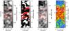 |
Fig. 1 Overview of the observations. The panels from left to right are: Ba ii 4554 Å continuum intensity in units of its spatially averaged value; mask applied to locate granules and intergranular lanes; Ba ii 4554 Å line center intensity in units of its spatially averaged value; magnetic field strength from the inversion of Fe i IR lines. Contours (same in all panels) mark the locations of granular areas with the magnetic field above 1.2 kG. |
Simultaneously with TIP-II, the TESOS instrument was making scans through the spectral profile of the Ba ii 4554 Å line. TESOS (Triple Etalon SOlar Spectrometer; Tritschler et al. 2002) is a Fabry-Perot interferometer equipped with three etalons that allow one to scan spectral lines in a two-dimensional field of view. The CCD of TESOS had 512 × 512 pixels of 0089 size. Thus, the total size of the observable area on the Sun was  . The Ba ii 4554 Å line was covered by 37 spectral points with a spectral sampling of 16 mÅ. During the scan, TIP was moving the whole field of view of TESOS at steps of 035. However, at every moment of the observations, the area scanned by TIP and the field of view of TESOS overlapped. Each complete scan of the 37 spectral points of the Ba ii line profile took 25.6 s.
In addition to TIP and TESOS, we also recorded Ca ii K 3968 Å filtergrams with a pixel size of 0123, a temporal cadence of 4.93 seconds and a total field of view of 110′′ × 110′′.
The seeing conditions were good to moderate during the observations. The r0 parameter was around 10, indicating spatial resolution no more than 05 in the blue range of the spectrum at 4500 Å, and the resolution around 2′′ in the infrared. Owning to jumps of the adaptive optics (AO) system, the observed area was lost a few times during the observations and we could not completely recover its position. Therefore, we used only five strictly co-spatial TIP scans (from 2nd to 6th) for the analysis, with a total duration of 34min41s.
2.1. Data reduction
As a first step of the reduction process, the data from all three cameras (TIP, TESOS and Ca ii K) were corrected for the dark current and flat field, following the standard procedure. In addition, spectropolarimetric data from TIP were corrected for the instrumental polarization, calibrated and de-modulated to give Stokes I, Q, U and V profiles, using the standard reduction routines for this instrument.
We then performed the spatial alignment between all three data channels. Here we recall that TIP records all Stokes spectra simultaneously, but each spatial slit position is separated by 27.3 s in time. In contrast, TESOS records all spatial points simultaneously, but each spectral position is separated by 25.6/37 s in time. The alignment of these data was far from trivial.
Firstly, we compared the images of a reticle target, scanned during the observations by both instruments. From them we calculated the rotation angle and scaling factor to apply to the TESOS data to have the same orientation and spatial sampling as TIP. We then rotated and re-sampled the TESOS data accordingly. Secondly, we constructed “false” continuum Stokes I maps from TIP (keeping in mind that they are not strictly simultaneous in time), and continuum Ba ii images from TESOS. To make a better match, we artificially decreased the spatial resolution of the TESOS continuum maps to make it similar to the resolution of the TIP maps in the infrared. The TIP continuum image was “moved” over the TESOS continuum image to find the location with the best correlation. This has allowed us to align both images with a one-pixel precision of TIP (0185). The common area between both instruments had the size of  . A similar procedure was applied to the Ca ii K data, using Ba ii line core images as a reference to find the best correlation.
In summary, after all the reduction and alignment processes, our observational material consists of the following datasets:
-
Five TIP maps of Stokes spectra ofFe i linesat 1.56 μm, separated by 6min50s in time and
in size; -
Time series of Ba ii 4554 Å line spectra over a
area, co-spatial with TIP, with a temporal cadence of 25.6 s and a duration of 34min41s; -
Time series of Ca ii K filtergrams over
area, co-spatial with TIP and TESOS, with a temporal cadence of 4.93 s and the same duration as the TIP and TESOS series.
Figure 1 gives an example of the co-spatial maps of the continuum and line core intensity in the Ba ii line, the mask applied to select granular and intergranular areas, and the magnetic field strength derived from Fe i infrared (IR) spectra (see the details below). In the following we do not use Ca ii K data, but we retain the complete description of our observational dataset for a forthcoming paper. The comparison of the Ba ii line core intensity maps and magnetic field strength map shows that areas with a stronger magnetic field are, generally, brighter. The Ba ii line core intensity traces magnetic field concentrations in a similar way as the Ca ii K line.
2.2. Calculation of the magnetic field from IR Fe i lines
Stokes parameters of the Fe i 15648 and 15652 Å lines were inverted using the SIR inversion code (Stokes Inversion based on Responce functions, see Ruiz Cobo & del Toro Iniesta 1992). We fitted all four Stokes parameters of the two Fe i lines. We assumed a one-component model including magnetic field. The free parameters of the inversion were temperature (with a maximum of five nodes), line of sight and microturbulent velocities, and magnetic field. The latter was assumed vertical and constant with height. The contribution of a non-magnetic surrounding was taken into account by varying the stray light fraction. An average Stokes I profile over the non-magnetic areas was taken as a stray light profile. The rightmost panel of Fig. 1 gives the magnetic field strength of the first (of the five) TIP maps used in the current study. The observed facular region contained features with quite strong magnetic field. Indeed, the magnetic field strength measured directly from the splitting of the infrared Fe i lines was very close to the one obtained from the inversion. The average stray light factor reached about 30%, and the average flux over the area was about 300 G. The histogram of the magnetic field strength measured in all spatial points in the five TIP scans is given in Fig. 2 (left panel). While there are many pixels with intermediate field strength (300−800 G), the histogram peaks at 1300 G.
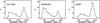 |
Fig. 2 Histograms of the magnetic field strength from the inversion of the Fe i lines. Left: histogram over all spatial points; middle: only pixels with a Ba ii continuum contrast higher than the average (granules); right: only pixels with a Ba ii continuum contrast lower than the average (intergranular lanes). |
2.3. Calculation of the velocity and intensity variations from Ba ii
The velocity and intensity variations were calculated from the Ba ii line profiles following the λ-meter technique (see for a detailed description Stebbins & Goode 1987; Shchukina et al. 2009; Kostik et al. 2009). As follows from Shchukina et al. (2009), the formation height of Ba ii line spans the entire photosphere from 0 to almost 700 km.
We used 14 reference widths of the average Ba ii 4554 Å line intensity profile over the whole time and space. For this average profile, and for prescribed line widths, W, we calculated the intensity value,  , and the displacements (velocities) in the red and blue wing,
  and
and  , corresponding to each width W. We repeated the same procedure for each individual Ba ii profile at each spatial position and time moment t. We then found intensity variations δI(t,x,W) and red and blue wing velocities Vr(t,x,W), Vb(t,x,W) at the corresponding 14 reference widths. We are interested in fluctuations of these quantities given by the following relations:
 ![Mathematical equation: \begin{eqnarray} \label{velo} \delta I(t,x,W) & = & I(t,x,W) - \bar{I}(W) \nonumber\\[1.5mm] \delta V_{\rm r}(t,x,W) & = & V_{\rm r}(t,x,W) - \bar{V_{\rm r}}(W) \nonumber\\[1.5mm] \delta V_{\rm b}(t,x,W) & = & V_{\rm b}(t,x,W) - \bar{V_{\rm b}}(W). \end{eqnarray}](/articles/aa/full_html/2012/09/aa19534-12/aa19534-12-eq26.png) (1)The intensity variations are normalized to their corresponding mean value for each W level, to give the contrast variations, δC, as
(1)The intensity variations are normalized to their corresponding mean value for each W level, to give the contrast variations, δC, as  (2)We recall that applying the λ-meter technique, both intensity (contrast) and velocity fluctuate for a given fixed reference width W, since this width can correspond to a higher or lower section of the profile, and can be displaced in wavelength due to velocities.
The zero velocity reference was placed requesting ⟨ δVr(t,x,W) ⟩ = 0 and ⟨ δVb(t,x,W) ⟩ = 0, averaged over time and space for the reference width W closest to the line core. This determination of zero velocity reference is less affected by the standard convective blueshift than a granulation-averaged intensity profile, because to first order the granular intensity-velocity correlation does not influence the averaged line minimum, as long as the granulation is resolved. According to several studies (e.g. Lopresto & Pierce 1985), the lines, forming high in the atmosphere (near the temperature minimum, as our Ba ii line) have very little convective blueshift. The above cited work does not provide information about the Ba ii 4554 Å line, but for lines formed at similar heights (Fe i 3767 Å, Na i 5896 Å, K i 7699 Å), the remaining blueshift is about 60 m s-1. Because of this, we realize that our determination of the zero velocity position may contain a blueshift, but its value is not expected to be higher than 60 m s-1.
We recall that the formation heights of the blue and red wing intensity points of the line profile are, in general, not the same because of the Doppler velocity shift (Shchukina et al. 2009), therefore the red and blue velocities may correspond to different heights. Despite this, in the rest of the paper we use average velocities:  (3)The formation heights corresponding to each width level are expected to vary significantly in space, being different in granules and intergranular lanes. To ascribe an approximate formation height to each of the 14 W levels, we followed NLTE (non-Local Thermodynamic Equilibrium) radiative transfer calculations, described in previous works (Shchukina et al. 2009; Kostik et al. 2009). In the following, we will refer to “continuum” velocity and “continuum” intensity (contrast) in Ba ii as velocities and intensities corresponding to the highest part of the profile, i.e., the deepest layer in the atmosphere sampled by our procedure. Throughout we adopt a positive sign for upflowing velocity (motion toward the observer).
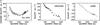 |
Fig. 3 Convective velocities measured in the Ba ii line as a function of magnetic field strength obtained from the Fe i lines. Left panel: unsigned values of the velocity, all pixels are considered. The three group of points correspond to the velocities at three levels of the Ba ii profile, larger points mean higher in the atmosphere (0, 400 and 650 km, approximately). Middle: only granular points, velocities at the deepest level of the atmosphere. Right panel: only intergranular points. |
2.4. Separation of convective and wave components
Variations of intensity δI(t,x,W) and velocities δV(t,x,W) are mainly caused by oscillatory and convective motions. Since here we are primary interested in convection, we filtered out oscillatory motions in the Fourier space based on the k−ω diagram (Khomenko et al. 2001; Kostik & Khomenko 2007; Kostik et al. 2009).
2.5. Separation into granules and intergranular lanes
We fragmented all spatial points into granular and intergranular points using as a criterion their continuum intensity in the Ba ii line. We removed from the consideration the dark pores (located mostly in intergranular lanes). Intergranular bright points, characteristic for facular areas at high spatial resolution (e.g. at 01), are not distinguishable at the resolution of our observations (see Fig. 1). The second right panel of this figure gives an example of the applied granular mask.
3. Results
To study the relationship between the magnetic field, velocity and intensity in our data we proceeded in the following way. The magnetic field values, measured in all pixels and in all five maps, were sorted by their magnitude, and then divided into 20 groups (or bins), each of them containing an equal number of pixels. Each bin was assigned a value of the magnetic field strength by averaging the B values over all points it contains. The Ba ii intensity and velocity values (at different levels of the profile) were measured and averaged separately for each group. In addition to that, we have performed a similar procedure, but separately for granular and intergranular points, previously segmented from all data.
Figure 3 (left panel) shows values of the unsigned convective velocities observed in Ba ii line at different heights in the solar atmosphere, binned for intervals of varying magnetic field strength. The dependence on the magnetic field strength is not monotonic. The velocity initially decreases with increasing magnetic field strength, reaching a minimum near B = 1000 G, and then increases again. A similar behavior of the velocities is observed at all 14 levels of the Ba ii line profile. For clearer view, the figure only presents data for three levels, corresponding, approximately, to heights of 0, 400, and 650 km. Note that unsigned velocities are represented and, accordingly, this behavior is not surprising. It can be easily understood in terms of magneto-convection, taking as example the behavior of the quiet-Sun internetwork magnetic fields (e.g., Khomenko et al. 2003, see their Fig. 7). Indeed, because our observations are taken close to the disk center, the unsigned (absolute) values of the vertical velocities are expected to be higher in granules (with weaker field) and in intergranular lanes (generally containing strong magnetic field concentrations), while they are low at the transition between granules and lanes (where the field is of intermediate strength). The existence of regions with almost zero component of the vertical velocity at the transitions between granules and lanes was recently reported from the quiet-Sun data taken by the IMaX/Sunrise instrument (Martínez Pillet et al. 2011), see Khomenko et al. (2010).
The middle and right panels of Fig. 3 show the behavior of the Ba ii velocities separately for granules and lanes, this time only for the deepest “continuum” atmospheric layer and taking into account their sign. As can be seen, upward velocities of granules decrease with increasing magnetic field strength, and the downward velocities in intergranular lanes are increasing, in agreement with what was said above.
Figure 4 shows the contrast variation measured at the deepest “continuum” atmospheric layer from the Ba ii profile binned for magnetic field intervals of varying strength. The contrast is defined as a standard deviation of the fluctuations of the quantity δC, see Eq. (2). Here we compare three different statistics: (1) all pixels are considered (black dots); (2) only granular points are considered (stars); and (3) only intergranular points are considered (open circles). The contrast is given in per cent with respect to the mean value over the whole observed area and time, so that dark areas have negative contrast and bright areas have positive contrast. In general, in all cases, the contrast decreases with magnetic field strength. When considering all points, the contrast changes from positive to negative as the magnetic field strength increases. The reason is similar to the case of velocities, i.e. brighter granules generally have a weaker field than darker intergranular lanes, same as for the magnetic fields in the quiet Sun. At the same time, it is interesting that the dependence on contrast becomes much weaker if we consider statistics separately for granules and lanes. For lanes, the dependence is within the error bar limit, meaning that the contrast of intergranular lanes is nearly independent of the field strength. We will discuss the implications of this finding in Sect. 4.
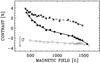 |
Fig. 4 Convective contrast measured from the Ba ii line at the deepest atmospheric layer as a function of magnetic field strength from Fe i lines. Black dots: all pixels are considered; stars: only granular points; open circles: only intergranular points. |
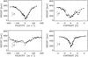 |
Fig. 5 Upper panels: height of the velocity sign reversal as a function of “continuum” velocity (left) and “continuum” contrast (right) from the Ba ii profile. The mean value is 330 ± 160 km. Each symbol is an average over a bin with an equal number of data points. Bottom panels: height of the contrast sign reversal as a function of the “continuum” velocity (left) and “continuum” contrast (right) from the Ba ii profile. The average value is 420 ± 130 km. |
Another known feature of solar granulation in the quiet non-magnetic areas is its contrast sign reversal and the velocity direction reversal observed at the middle photosphere. Here we investigate this feature, but for the facular area, searching for dependences of the heights of reversal on the strength of granular motions at the continuum formation level, similar to Kostik et al. (2009).
In our data, only about 37% of elements show the contrast reversal with height, and 26% show the reversal of the direction of motion, as calculated from the Ba ii λ-meter velocities and intensities. We only used these elements for the results presented in Fig. 5. The scatter of heights of the velocity and contrast sign reversals is very high. These heights vary in a range from 50 to 650 km, i.e. spanning almost the whole formation height range of the Ba ii line profile. Nevertheless, if these heights are plotted as a function of “continuum” velocity or “continuum” contrast, there is a clear dependence, similar to the case of the quiet-Sun Ba ii line data used in Kostik et al. (2009). Figure 5 shows this result. We calculate the error bars as a standard deviation over the values for each bin, and then averaged over all bins. The larger is the continuum velocity and contrast of convective elements, the larger is the height where they change their direction of motion (upper two panels). On average, this height is about 330 ± 160 km. Same happens for the contrast sign reversal (bottom two panels). The dependence on the continuum contrast is more pronounced than on the velocity. On average, the contrast sign reversal of the convective elements takes place at about 420 ± 130 km. Interestingly, both average reversal heights are about 100 km larger than in the quiet-Sun data of Kostik et al. (2009) ( ≈ 210 and ≈ 330 km, compared to 330 and 420 km).
Both the statistics over the quiet-Sun data of Kostik et al. (2009), and the facular data in the present study suggest that the velocity sign reversal happens at lower heights than the contrast sign reversal. This should not be interpreted in a way that the same ascending element first changes the direction of motion at one height h1 and then the contrast at another height h2, where h1 < h2. We made the statistics for the contrast and velocity sign reversals independently. According to this, we can have independent elements, one changing the direction of motion at h1 and another one changing the contrast at h2. Also, the descending elements can first change their contrast and then the direction of motion at a lower height. We did not differentiate between the descending and ascending elements, nor between the bright and dark elements when calculating the reversal heights. Note also that only low percentage of elements reverse their contrast and direction of motion in our data.
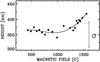 |
Fig. 6 Heights of the velocity and contrast sign reversal as a function of magnetic field strength. |
Our next step was to investigate if the reversal height depends on the magnetic field strength. To increase the statistics, we averaged together velocity and contrast reversal heights in all data points for bins of varying magnetic field strength. The result is given in Fig. 6. Obviously, there is a hint for such a dependence within the error bar limit. The reversal height is roughly independent of the magnetic field strength till about 1000 G. For the higher field strengths, the reversal height increases from about 350 to 430 km.
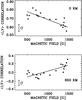 |
Fig. 7 Top: correlation coefficient between the “continuum” intensity and “continuum” velocity measured from the Ba ii line profiles as a function of the magnetic field strength. Bottom: same for the velocities and intensities at the highest level ~650 km. |
Yet another important parameter characterizing granulation is the correlation between intensity (contrast) and velocity of granular elements. This correlation is expected to be maximum at the continuum formation layer, decreasing to zero in the middle photosphere (see e.g., Kostyk & Shchukina 2004, and references therein). The values of the correlation measured by these authors do not exceed 75% even in the deepest layer, meaning that total coincidence of the intensity and velocity maxima is rare for the solar photosphere. Here we investigate how the correlation coefficient between the velocity and intensity changes as a function of the magnetic field. Figure 7 shows this dependence for the two atmospheric levels: the deepest “continuum” levels (top) and the highest level around the Ba ii line core (~650 km, bottom). Apparently, at the “continuum” level the correlation is maximum for the intermediate values of the magnetic field strength (500−700 G), reaching as high as 77%. The correlation coefficient decreases to 60% as the magnetic field increases. The variations between the maximum and minimum values are larger than the statistical error bar (also shown in the figure). Unlike that, the correlation at 650 km is negative for the intermediate magnetic field strength, which is characteristic for inverse granulation. For higher field strengths above 1000 G, the correlation turns positive and reaches 20% at maximum. This result indicates that a strong magnetic field in facular areas helps to preserve the structure of convective elements till higher heights.
4. Discussion
Before discussing our results, we recall the medium spatial resolution (~05 in the blue part of the spectrum) of our observational data which, in principle, could affect our results. In particular, we do not “see” manifestations of strong kG magnetic field concentrations expected to be appear as bright points (BPs) in intergranular lanes (Title et al. 1992; Berger et al. 2004; Narayan & Scharmer 2010). Therefore, there might be a chance that after segmenting all data points into granular and intergranular points, unresolved BPs may appear belonging to either granular or intergranular groups, depending on the atmospheric blurring. Possibly, the second maximum (B = 1300 G) on the histogram of the magnetic field strength distribution over granules (Fig. 2, middle panel) is due to such unresolved BPs. For the purpose of visual comparison, the granular pixels with magnetic field above 1.2 kG are marked red in Fig. 1. At least visually, there is nothing particular about the location of these pixels. To check if the unresolved BPs affect our results, we repeated all the relevant calculations presented above, but this time excluding the granular points with a magnetic field strength above 1.1 kG (a value corresponding to a local minimum on the histogram in Fig. 2, middle panel). We found no significant differences in our results.
The dependence of convective velocities on the magnetic field strength can be compared to the results of similar studies by other authors. Measurements for the plage and facular areas are not that frequent and the most adequate comparison can be made with the works of Title et al. (1992); Montagne et al. (1996); Morinaga et al. (2008); Narayan & Scharmer (2010). These authors used different method to obtain the magnetic field strength from their measurements (inversion of spectropolarimetric data or magnetogram signals). Also, data of different spatial resolution (between 015 and 10) and at different wavelengths (spectral lines from 4305 Å to 6768 Å) are presented. Consequently, a direct one-to-one comparison with our results is not possible. Nevertheless, we can state that there is a qualitative agreement between our results and those from the works mentioned above for the velocity distributions. The granular motions in plage areas on average exhibit upflows for intermediate field strength below 600 G. For the stronger fields above 600 G the structures show a tendency for downflows (except for Title et al. 1992, where downflows are dominant for the magnetogram signal above 100 G). Our results presented in Fig. 3 better agree with the results by Morinaga et al. (2008), though these authors studied the velocity flows in the vicinity of a solar pore, unlike the quiet plage analyzed here.
Evans & Catalano (1972) and Holweger & Kneer (1989) were apparently the first ones to discover the contrast sign reversal with height in the solar atmosphere. Later, this phenomenon was investigated by Kuc˘era et al. (1995), Espagnet et al. (1995), Kostyk & Shchukina (2004), Puschmann et al. (2005), Stodilka (2006), Janssen & Cauzzi (2006). Cheung et al. (2007) have shown from numerical MHD simulations that the temperature (and hence contrast) reversal in the photosphere is due to the competition between expansion and cooling of rising fluid elements and their radiative heating. The heights of contrast reversal derived from observations by different authors vary in a wide range from 60 to 350 km. Kostik et al. (2009) pointed out that this scatter may be attributed to the difference in the formation heights of the spectral lines used in different observational studies. More recently, it was found that not only contrast reverses sign in the solar atmosphere, but also the direction of motion of convective elements reverses with height (Kostyk & Shchukina 2004; Kostik et al. 2009). These studies were performed for granulation observed in very quiet non-magnetic regions. Our results from Fig. 5 point out that both contrast and velocity sign reversal take place in the facular regions as well. The moderate magnetic field in faculae (400−900 G) does not affect the height where the reversal takes place compared to the quiet solar regions (Fig. 6). However, the stronger field above 1 kG “forces” the convective elements to travel over longer vertical distances without changing the sign of contrast and direction of motion. Apparently, strong magnetic field in facular areas promotes more effective energy transfer in the upper layers of the solar atmosphere by convective elements, since they can reach greater heights. At first glance, it might seem that this conclusion disagrees with the results shown in the top panel of Fig. 7 regarding the correlation between velocity and contrast. The correlation coefficient almost linearly decreases with increasing magnetic field. However, the correlation at the heights of formation of the Ba ii line core behaves in the opposite way (bottom panel of Fig. 7). While the absolute values of the correlation in the upper atmosphere are lower, as expected, the correlation is, on average, positive for stronger magnetic field strengths above 1 kG, indicating that the structure of convective elements is maintained up to that height.
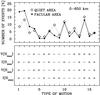 |
Fig. 8 Convective motions in the solar atmosphere according to 16-column model. Upper panel shows the number of cases corresponding to each of the 16 types of motions (as defined at the bottom panel) between 0 and 650 km. |
Yet another proof of this result is provided by Fig. 8. This figure compares the types of motion observed in the quiet area (data from Kostik et al. 2009) and in our facular area. The bottom panel of the figure indicates our classification of the types of motion: sign “+” indicates convective elements moving upward or those whose contrast is above the average; sign “−” indicats downward moving elements or those with the contrast below the average. We compare the velocity sign and contrast of convective elements at the “continuum” level and the at highest level available for us around the formation of the Ba ii line core. Interestingly, we find that the number of convective elements that do not change contrast and velocity direction in the facular area is about 53% (motions of type 1 to 4). Compared to this, in the quiet area only 31% of the convective elements behave this way. We conclude that the strong magnetic field of the facular region helps to stabilize the convective elements and allows the convective energy to reach greater heights.
Possibly the most interesting result of our study is presented in Fig. 4. The general decrease of the contrast with increasing magnetic field (if all points are considered equally) seems to be a natural result and confirms the results of the earlier studies (Title et al. 1992; Topka et al. 1992; Montagne et al. 1996; Topka et al. 1997; Berger et al. 2007; Kobel et al. 2011). However, the behavior of intergranular pixels, considered separately from the rest, is significantly different (dashed line in Fig. 4). Namely, the intergranular contrast is essentially independent of the magnetic field strength within the error bar limit. The same conclusion was reached previously by Berger et al. (2007). The authors claimed that in facula regions close to the limb one rather detects granular walls, which should be essentially independent of the magnetic field strength. Here we confirm this finding but for the facular region close to the disk center.
The decrease of the contrast with increasing magnetic field obtained in previous studies seems to be a result of the particular distribution of the magnetic field strength in these structures (Fig. 2). The granules have generally weaker fields, while intergranules have stronger ones. By averaging all the intensity values for different B intervals, one would naturally obtain more granular pixels for the bins with lower B (i.e., higher contrast) and the opposite for intergranules. Therefore, it is important to segment granular and intergranular pixels prior to analyzing the dependence of the contrast on B.
All statistical dependences found in our paper are more significant that the corresponding error bars, given in all the figures. The only exception is the dependence shown in Fig. 6, which is within the error bar. The error bars were calculated as standard deviation over the values averaged for a given bin.
The advantage of our work over similar studies is the real magnetic field measurements obtained from the inversion of extremely magnetically sensitive Fe i spectra in the infrared, instead of using a magnetogram signal. The alignment of our data sets from both instruments was performed with a one-pixel precision (0185), improving the statistical significance of our results. It is important to recall, however, that the diffraction limits in the visible and in the infrared are very different, leading to a naturally lower spatial resolution of the infrared data. For a better alignment we artificially reduced the spatial resolution of the continuum Ba ii maps to make it comparable with that of TIP Stokes I maps. The lower resolution of TIP data might in principle affect the precise value of the magnetic field derived from this data, since the magnetic field patches are more diffused and magnetic elements of mixed polarities might cancel. However, the cancelations are expected to be more important in the mixed-polarity inter-network areas, and not in a (mostly unipolar) plage area such as the observed one. Since we derived the magnetic field from the inversion of Stokes profiles, using a stray-light component as a free parameter, this improves our accuracy in the magnetic field strength determination. The magnetic field values given at the horizontal axis of Figs. 3, 4, 6, and 7 are averages over the intensity bins. While these average values might, in principle, be affected by the cancelations in a mixed-polarity area, we do not expect this to be important in a uni-polar plage. Another possible source of error is that our data do not have a sufficiently high resolution to resolve intergranular bright points. However, as pointed out at the beginning of this section, we have cross-checked that removing the “granular” points with B > 1.2 kG from our analysis (as possible unresolved bright points) provides the same results, in particular the one given in Fig. 4. This confirms once more our conclusion that the contrast of intergranular lanes is independent of the magnetic field, in agreement with Berger et al. (2007).
It will be interesting in the future to check the results of our work using data with a higher spatial resolution and maintaining the advantages of the simultaneous Stokes polarimetry and velocity/intensity measurements up to the upper photosphere.
5. Conclusions
Using simultaneous spectropolarimetric observations in the infrared Fe i lines at 1.56 μm and spectral observations of the strong line of Ba ii 4554 Å formed high in the atmosphere, with a moderate temporal resolution, we investigated the behavior of the convective component of the intensity and velocity fields in the facular region close to the solar disk center. The Ba ii line allowed us to perform a study over a wide range of heights, from the continuum formation height up to about 650 km in the solar atmosphere. We have reached the following conclusions:
-
At the bottom of the photosphere, the convective velocities ofgranules decrease with magnetic field strength, while theconvective velocities of intergranules increase with magneticfield strength.
-
Similar to the quiet regions, we detected that in facular regions the contrast of granulation and the velocities of convective elements reverse their sign with height. The height at which this reversal takes place depends on the strength of convective elements at the bottom of the photosphere, but also on the magnetic field strength. Convective elements above stronger magnetic features reach higher into the atmosphere without breaking.
-
The correlation coefficient between velocity and intensity at the bottom-most level decreases with the magnetic field. In the upper atmosphere, above 500 km, the correlation increases with increasing the magnetic field.
-
The contrast of convective elements decreases with increasing magnetic field strength. But if intergranular lanes are considered separately, their contrast is nearly independent of the field strength.
Acknowledgments
Based on observations made with the VTT telescope operated on the island of Tenerife by the Kiepenheuer-Institut fur Sonnenphysik in the Spanish Observatorio del Teide of the Instituto de Astrofisica de Canarias. This research has been supported by the Spanish Ministry of Economy and Competitiveness (MINECO) under the grants AYA2010-18029 and AYA2011-24808. The authors are grateful to Manuel Collados for the help with observations and useful discussions.
References
- Auffret, H., & Muller, R. 1991, A&A, 246, 264 [NASA ADS] [Google Scholar]
- Berger, T. E., Rouppe van der Voort, L. H. M., Löfdahl, M. G., et al. 2004, A&A, 428, 613 [NASA ADS] [CrossRef] [EDP Sciences] [Google Scholar]
- Berger, T. E., Title, A. M., Tarbell, T., et al. 2007, in New Solar Physics with Solar-B Mission, eds. K. Shibata, S. Nagata, & T. Sakurai, ASP Conf. Ser., 369, 103 [Google Scholar]
- Carlsson, M., Stein, R. F., Nordlund, Å., & Scharmer, G. B. 2004, ApJ, 610, L137 [NASA ADS] [CrossRef] [Google Scholar]
- Cheung, M. C. M., Schüssler, M., & Moreno-Insertis, F. 2007, A&A, 461, 1163 [NASA ADS] [CrossRef] [EDP Sciences] [Google Scholar]
- Cheung, M. C. M., Schüssler, M., Tarbell, T. D., & Title, A. M. 2008, ApJ, 687, 1373 [NASA ADS] [CrossRef] [Google Scholar]
- Collados, M., Lagg, A., Díaz Garcí A, J. J., et al. 2007, in The Physics of Chromospheric Plasmas, eds. P. Heinzel, I. Dorotovič, & R. J. Rutten, ASP Conf. Ser., 368, 611 [Google Scholar]
- de Boer, C. R., Stellmacher, G., & Wiehr, E. 1997, A&A, 324, 1179 [NASA ADS] [Google Scholar]
- Espagnet, O., Muller, R., Roudier, T., et al. 1995, A&AS, 109, 79 [NASA ADS] [Google Scholar]
- Evans, J. W., & Catalano, C. P. 1972, Sol. Phys., 27, 299 [NASA ADS] [CrossRef] [Google Scholar]
- Hirzberger, J., & Wiehr, E. 2005, A&A, 438, 1059 [NASA ADS] [CrossRef] [EDP Sciences] [Google Scholar]
- Holweger, H., & Kneer, F. 1989, in Solar and Stellar Granulation, eds. R. J. Rutten, & G. Severino, Proc. 3rd International Workshop of the Astronomical Observatory of Capodimonte, NATO Adv. Sci. Instit. (ASI) Ser. C (Dordrecht: Kluwer), 263, 173 [Google Scholar]
- Janssen, K., & Cauzzi, G. 2006, A&A, 450, 365 [NASA ADS] [CrossRef] [EDP Sciences] [Google Scholar]
- Keller, C. U., Schüssler, M., Vögler, A., & Zakharov, V. 2004, ApJ, 607, L59 [NASA ADS] [CrossRef] [Google Scholar]
- Khomenko, E. V., Kostik, R. I., & Shchukina, N. G. 2001, A&A, 369, 660 [NASA ADS] [CrossRef] [EDP Sciences] [Google Scholar]
- Khomenko, E. V., Collados, M., Solanki, S. K., et al. 2003, A&A, 408, 1115 [NASA ADS] [CrossRef] [EDP Sciences] [Google Scholar]
- Khomenko, E., Martínez Pillet, V., Solanki, S. K., et al. 2010, ApJ, 723, L159 [NASA ADS] [CrossRef] [Google Scholar]
- Kostik, R. I., & Khomenko, E. V. 2007, A&A, 476, 341 [NASA ADS] [CrossRef] [EDP Sciences] [Google Scholar]
- Kostik, R., Khomenko, E., & Shchukina, N. 2009, A&A, 506, 1405 [NASA ADS] [CrossRef] [EDP Sciences] [Google Scholar]
- Kostyk, R., & Shchukina, N. 2004, Astron. Rep., 48, 769 [Google Scholar]
- Kobel, P., Solanki, S. K., & Borrero, J. M. 2011, A&A, 531, A112 [NASA ADS] [CrossRef] [EDP Sciences] [Google Scholar]
- Kučera, A.,Rybák, J., & Wöhl, H. 1995, A&A, 298, 917 [NASA ADS] [Google Scholar]
- Lites, B. W., Scharmer, G. B., Berger, T. E., & Title, A. M. 2004, Sol. Phys., 221, 65 [NASA ADS] [CrossRef] [Google Scholar]
- Lopresto, J. C., & Pierce, A. K. 1985, Sol. Phys., 102, 21 [NASA ADS] [CrossRef] [Google Scholar]
- Martínez Pillet, V., Del Toro Iniesta, J. C., Álvarez-Herrero, A., et al. 2011, Sol. Phys., 268, 57 [NASA ADS] [CrossRef] [Google Scholar]
- Montagne, M., Mueller, R., & Vigneau, J. 1996, A&A, 311, 304 [NASA ADS] [Google Scholar]
- Morinaga, S., Sakurai, T., Ichimoto, K., et al. 2008, A&A, 481, L29 [NASA ADS] [CrossRef] [EDP Sciences] [Google Scholar]
- Muller, R. 1977, Sol. Phys., 52, 249 [NASA ADS] [CrossRef] [Google Scholar]
- Narayan, G., & Scharmer, G. B. 2010, A&A, 524, A3 [NASA ADS] [CrossRef] [EDP Sciences] [Google Scholar]
- Nesis, A., & Mattig, W. 1989, A&A, 221, 130 [NASA ADS] [Google Scholar]
- Okunev, O. V., & Kneer, F. 2004, A&A, 425, 321 [NASA ADS] [CrossRef] [EDP Sciences] [Google Scholar]
- Okunev, O. V., & Kneer, F. 2005, A&A, 439, 323 [NASA ADS] [CrossRef] [EDP Sciences] [Google Scholar]
- Ortiz, A., Solanki, S. K., Domingo, V., Fligge, M., & Sanahuja, B. 2002, A&A, 388, 1036 [NASA ADS] [CrossRef] [EDP Sciences] [Google Scholar]
- Puschmann, K. G., Ruiz Cobo, B., Vázquez, M., Bonet, J. A., & Hanslmeier, A. 2005, A&A, 441, 1157 [NASA ADS] [CrossRef] [EDP Sciences] [Google Scholar]
- Rimmele, T. R. 2004, ApJ, 604, 906 [NASA ADS] [CrossRef] [Google Scholar]
- Ruiz Cobo, B., & del Toro Iniesta, J. C. 1992, ApJ, 398, 375 [NASA ADS] [CrossRef] [Google Scholar]
- Schmidt, W., Grossmann-Doerth, U., & Schroeter, E. H. 1988, A&A, 197, 306 [NASA ADS] [Google Scholar]
- Shchukina, N., Olshevsky, V., & Khomenko, E. 2009, A&A, submitted [Google Scholar]
- Spruit, H. C. 1976, Sol. Phys., 50, 269 [NASA ADS] [CrossRef] [Google Scholar]
- Stebbins, R. T., & Goode, P. R. 1987, Sol. Phys., 110, 237 [NASA ADS] [CrossRef] [Google Scholar]
- Steiner, O. 2005, A&A, 430, 691 [NASA ADS] [CrossRef] [EDP Sciences] [Google Scholar]
- Stodilka, M. 2006, Kinematika i Fizika Nebesnich Tel, 22, 173 [NASA ADS] [Google Scholar]
- Sütterlin, P., Wiehr, E., & Stellmacher, G. 1999, Sol. Phys., 189, 57 [NASA ADS] [CrossRef] [Google Scholar]
- Title, A. M., Topka, K. P., Tarbell, T. D., et al. 1992, ApJ, 393, 782 [NASA ADS] [CrossRef] [Google Scholar]
- Topka, K. P., Tarbell, T. D., & Title, A. M. 1992, ApJ, 396, 351 [NASA ADS] [CrossRef] [Google Scholar]
- Topka, K. P., Tarbell, T. D., & Title, A. M. 1997, ApJ, 484, 479 [NASA ADS] [CrossRef] [Google Scholar]
- Tritschler, A., Schmidt, W., Langhans, K., & Kentischer, T. 2002, Sol. Phys., 211, 17 [NASA ADS] [CrossRef] [Google Scholar]
- Vögler, A. 2005, Mem. Soc. Astron. Italiana, 76, 842 [Google Scholar]
All Figures
|
Fig. 1 Overview of the observations. The panels from left to right are: Ba ii 4554 Å continuum intensity in units of its spatially averaged value; mask applied to locate granules and intergranular lanes; Ba ii 4554 Å line center intensity in units of its spatially averaged value; magnetic field strength from the inversion of Fe i IR lines. Contours (same in all panels) mark the locations of granular areas with the magnetic field above 1.2 kG. |
| In the text | |
|
Fig. 2 Histograms of the magnetic field strength from the inversion of the Fe i lines. Left: histogram over all spatial points; middle: only pixels with a Ba ii continuum contrast higher than the average (granules); right: only pixels with a Ba ii continuum contrast lower than the average (intergranular lanes). |
| In the text | |
|
Fig. 3 Convective velocities measured in the Ba ii line as a function of magnetic field strength obtained from the Fe i lines. Left panel: unsigned values of the velocity, all pixels are considered. The three group of points correspond to the velocities at three levels of the Ba ii profile, larger points mean higher in the atmosphere (0, 400 and 650 km, approximately). Middle: only granular points, velocities at the deepest level of the atmosphere. Right panel: only intergranular points. |
| In the text | |
|
Fig. 4 Convective contrast measured from the Ba ii line at the deepest atmospheric layer as a function of magnetic field strength from Fe i lines. Black dots: all pixels are considered; stars: only granular points; open circles: only intergranular points. |
| In the text | |
|
Fig. 5 Upper panels: height of the velocity sign reversal as a function of “continuum” velocity (left) and “continuum” contrast (right) from the Ba ii profile. The mean value is 330 ± 160 km. Each symbol is an average over a bin with an equal number of data points. Bottom panels: height of the contrast sign reversal as a function of the “continuum” velocity (left) and “continuum” contrast (right) from the Ba ii profile. The average value is 420 ± 130 km. |
| In the text | |
|
Fig. 6 Heights of the velocity and contrast sign reversal as a function of magnetic field strength. |
| In the text | |
|
Fig. 7 Top: correlation coefficient between the “continuum” intensity and “continuum” velocity measured from the Ba ii line profiles as a function of the magnetic field strength. Bottom: same for the velocities and intensities at the highest level ~650 km. |
| In the text | |
|
Fig. 8 Convective motions in the solar atmosphere according to 16-column model. Upper panel shows the number of cases corresponding to each of the 16 types of motions (as defined at the bottom panel) between 0 and 650 km. |
| In the text | |
Current usage metrics show cumulative count of Article Views (full-text article views including HTML views, PDF and ePub downloads, according to the available data) and Abstracts Views on Vision4Press platform.
Data correspond to usage on the plateform after 2015. The current usage metrics is available 48-96 hours after online publication and is updated daily on week days.
Initial download of the metrics may take a while.