| Issue |
A&A
Volume 536, December 2011
|
|
|---|---|---|
| Article Number | A61 | |
| Number of page(s) | 13 | |
| Section | Planets and planetary systems | |
| DOI | https://doi.org/10.1051/0004-6361/201117558 | |
| Published online | 08 December 2011 | |
The rotation of Mimas
1
FUNDP-University of NamurDepartment of Mathematics & NAmur
Center for Complex SYStems (NAXYS), Rempart de la Vierge 8, 5000
Namur,
Belgium
e-mail: benoit.noyelles@fundp.ac.be
2
IMCCE, Paris Observatory, UPMC, Univ. Lille 1, CNRS UMR
8028, 77 avenue Denfert
Rochereau, 75014
Paris,
France
3
Royal Observatory of Belgium, Ringlaan 3, 1180
Brussels,
Belgium
4
Université Pierre et Marie Curie Paris 6,
4 place Jussieu, 75005
Paris,
France
Received:
24
June
2011
Accepted:
27
September
2011
Context. The Cassini mission in the Saturnian system is an outstanding opportunity to improve our knowledge of the satellites of Saturn. The data obtained thanks to this mission must be balanced with theoretical models.
Aims. This paper aims at modelling the rotation of Mimas with respect to its possible internal structure.
Methods. We first built different interior models, considering Mimas to be composed of two rigid layers with different porosity. Then we simulated the rotational behaviour of these models in a three-degree of freedom numerical code, considering the complete ephemerides of a Mimas whose rotation is disturbed by Saturn. We also estimated the deviation of its longitudinal orientation caused by tides.
Results. We expect a signature of the internal structure up to 0.53° in the longitudinal librations and an obliquity between 2 and 3 arcmin, the exact values depend on the interior.
Conclusions. The longitudinal librations should be detectable, but inverting them to arrive at clues on the internal structure of Mimas is challenging.
Key words: planets and satellites: individual: Mimas / planets and satellites: interiors / celestial mechanics
© ESO, 2011
1. Introduction
The Cassini spacecraft gives us the unique opportunity to obtain an accurate set of geodetic data for the icy satellites of Saturn such as the shape, the gravitational field, and the rotational data (Thomas 2010). The flybys of Mimas have provided high-resolution images of the surface in the finest detail yet seen (Roatsch et al. 2009). The Cassini spacecraft has detected temperature inhomogeneities (Howett et al. 2011), which are usually attributed to exogenic processes. The theoretical model of Mimas’ rotational state can be used to interpret the Cassini data and to better understand its interior and evolution.
As our Moon, Mimas is in synchronous rotation with its planet and shows almost the same face towards Saturn. Moreover, it is considered to have a large librational amplitude (Comstock & Bills 2003). The rotational state of a synchronous body depends on the mass distribution of the body, and therefore it is a signature of its internal structure. Here, we propose to model the rotation of Mimas considering it as a rigid body. A highly rigid interior of Mimas for most of its history is consistent with its un-relaxed shape (Thomas et al. 2007; Thomas 2010).
Because the distant spacecraft flybys of Mimas do not allow the determination of the gravity field nor the gravity harmonics, the mass of Mimas is determined from an analysis of its orbital resonances with Tethys and Methone (Jacobson et al. 2006). But its internal structure remains uncertain. The mean density of 1.15 g cm-3 suggests that Mimas consists of a homogenous mixture of ice and rocks. The observed shape of Mimas by Voyager has been interpreted as an indication of interior mass concentration, which can be either caused by internal differentiation (Dermott & Thomas 1988) or radially variable porosity (Eluszkiewicz 1990). However, Cassini observations showed that Mimas’ shape, although a triaxial ellipsoid, deviates slightly from a hydrostatic shape and therefore an interpretation of the interior configuration from the shape is limited (Thomas et al. 2007; Thomas 2010). In the present study, we consider Mimas to be composed of two rigid layers. We consider a hydrostatic and a non-hydrostatic interior model. The interior models considering compaction of ice-silica particle mixtures (Yasui & Arakawa 2009) are expected to yield realistic principal moment of inertia A < B < C (Eluszkiewicz 1990). Because Mimas orbits close to its parent planet, the present-day diurnal tidal stresses can be significant, and we took the tidal effects into account as well.
The paper is structured as follows: we first model the internal structure of Mimas considering two different assumptions: that Mimas is in hydrostatic equilibrium, and that its ellipsoid of gravity is proportional to its ellipsoid of shape. From these two assumptions we derive 23 models of Mimas. Then we perform numerical integrations of the rotation of these “Mimases” in a full three-degree of freedom conservative models. Finally, we check the influence of the tides on the equilibrium orientation of Mimas’ long axis.
2. Internal structure
Interior structure models of planets and natural satellites are in general non-unique because one has fewer constraints than unknowns. For Mimas we have only two constraints: the mean radius R and the mean density ρ, or the mass m (Table 1). We are here concerned with the rotation, and accordingly the moment of inertia differences are the main point of interest.
Because we have only few constraints, we preferred a most simple interior structure for our models. We assumed a two-layer interior structure model with a rocky core and icy mantle. The models with a variable porosity, which is supported by recent compaction experiments (Yasui & Arakawa 2009), yield realistic moments of inertia (Eluszkiewicz 1990). The mean density of Mimas is close to the density of water ice and the interior is consistent with an icy mantle and a small rocky core; alternatively Mimas can be homogenous with a variable or constant porosity.
With Mimas’ figure departed from hydrostatic shape (Thomas et al. 2007; Thomas 2010) and without the knowledge of C22 and J2, we do not know the moment of inertia differences. As for the Moon (see e.g. Lambeck & Pullan 1980), the internal mass distribution could be a fossil shape that dates back from an earlier orbital position where the tidal heating was significant with higher orbital eccentricity and obliquity or a frozen shape following a large impact. Mimas shows a heavily cratered surface without signs of geological activity for billions of years. Its high free eccentricity gives another reason for low internal activity. This anomalously high eccentricity of Mimas can be explained by a passage through several past resonances (Meyer & Wisdom 2008). A determination of the gravity coefficients C22 and J2 = −C20 is necessary to conclude on the hydrostatic equilibrium because the figure of Mimas may not represent the real flattening or the internal mass determination, as is the case for Titan (Zebker 2009). As suggested by Johnson et al. (2006), large impact craters and heating of Mimas’ hemispheres by Saturn to different amounts may be potential sources of the considerable non-hydrostatic anomalies that could impede an accurate interpretation of the shape data.
2.1. Hydrostatic approximation
Because we do not know the gravity coefficients C22 and
J2, we used a simple approach. For a two-layer interior
model the core radius Rc can be determined if the densities of
the rocky core ρc and the icy mantle
ρs are known, i.e. 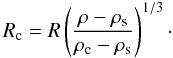 (1)The moment of
inertia factor
(MOI = Ip/(MR2))
is given as
(1)The moment of
inertia factor
(MOI = Ip/(MR2))
is given as 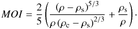 (2)Figure 1 shows that without additional constraints, plausible
density values of the core and icy shell yield
0.3 < MOI < 0.4. The range of the MOI was used to estimate
the moment of inertia of tri-axial Mimas, as shown below.
(2)Figure 1 shows that without additional constraints, plausible
density values of the core and icy shell yield
0.3 < MOI < 0.4. The range of the MOI was used to estimate
the moment of inertia of tri-axial Mimas, as shown below.
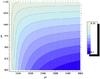 |
Fig. 1 Variations of the moment of inertia factor (MOI) with icy shell and rocky core densities. |
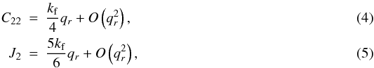
For a satellite in hydrostatic equilibrium, the MOI is related to the
fluid Love number kf, which describes the reaction of the
satellite to a perturbing potential after all viscous stresses have relaxed (Munk & MacDonald 1960; Hubbard & Anderson 1978): ![\begin{equation} \label{eq:moi} MOI=\frac{2}{3}\left[1-\frac{2}{5}\sqrt{\frac{4-k_{\rm f}}{1+k_{\rm f}}}\right], \end{equation}](/articles/aa/full_html/2011/12/aa17558-11/aa17558-11-eq20.png) (3)and the gravity
coefficients C22 and J2 are
determined from (Rappaport et al. 1997)
(3)and the gravity
coefficients C22 and J2 are
determined from (Rappaport et al. 1997)
 where
where
 ,
Ω being the spin velocity of Mimas, equal to its mean motion n because
Mimas is in synchronous rotation. With the numerical values given in Table 1, we have
qr = 0.01854.
,
Ω being the spin velocity of Mimas, equal to its mean motion n because
Mimas is in synchronous rotation. With the numerical values given in Table 1, we have
qr = 0.01854.
The differences between the three principal moments of inertia
A < B < C are
determined from the definitions of C22
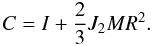
and J2, i.e. 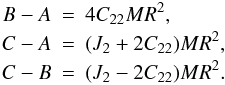 The
relationship between the mean moment of inertia
The
relationship between the mean moment of inertia  and the
polar moment of inertia C is
and the
polar moment of inertia C is
 (6)We can then calculate all
three moments of inertia A, B and C.
(6)We can then calculate all
three moments of inertia A, B and C.
Physical and dynamical properties of Mimas used in the calculations.
2.2. Nonhydrostatic shape
We here use the observed shape (a = 207.8 km,
b = 196.7 km, c = 190.6 km, Thomas 2010) to calculate the moments of inertia of Mimas, assuming
that the shape of the core is proportional to that of Mimas, i.e. we assume 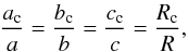 (7)where
ac, bc and
cc are the dimensions of the core, and
Rc its mean radius (Eq. (1)).
(7)where
ac, bc and
cc are the dimensions of the core, and
Rc its mean radius (Eq. (1)).
A quadrature over the volume of the core and the shell gives ![\begin{eqnarray} C_{\rm c} & = & \iiint_{\rm core}\rho_{\rm c}\left(x^2+y^2\right){\rm d}x\,{\rm d}y\,{\rm d}z \nonumber \\ & = & \frac{4}{15}\pi a_{\rm c}b_{\rm c}c_{\rm c}\left(a_{\rm c}^2+b_{\rm c}^2\right)\rho_{\rm c} \nonumber \\ & = & \frac{4}{15}\pi abc\left(a^2+b^2\right)\rho_{\rm c}\left(\frac{R_{\rm c}}{R}\right)^5, \label{eq:cc} \\ C_{\rm s} & = & \iiint_{\rm Mimas}\rho_{\rm s}\left(x^2+y^2\right){\rm d}x\,{\rm d}y\,{\rm d}z \nonumber \\ & & -\iiint_{\rm core}\rho_{\rm s}\left(x^2+y^2\right){\rm d}x\,{\rm d}y\,{\rm d}z \nonumber \\ & = & \frac{4}{15}\pi abc\left(a^2+b^2\right)\rho_{\rm c}\left[1-\left(\frac{R_{\rm c}}{R}\right)^5\right]\cdot\label{eq:cs} \end{eqnarray}](/articles/aa/full_html/2011/12/aa17558-11/aa17558-11-eq50.png) We
then obtain
C = Cc + Cs.
The other moments of inertia A and B being obtained
similarly, we have
We
then obtain
C = Cc + Cs.
The other moments of inertia A and B being obtained
similarly, we have ![\begin{eqnarray} A & = & \frac{4}{15}\pi abc\left(b^2+c^2\right)\left[\left(\rho_{\rm c}-\rho_{\rm s}\right)\left(\frac{R_{\rm c}}{R}\right)^5+\rho_{\rm s}\right], \label{eq:ga} \\ B & = & \frac{4}{15}\pi abc\left(a^2+c^2\right)\left[\left(\rho_{\rm c}-\rho_{\rm s}\right)\left(\frac{R_{\rm c}}{R}\right)^5+\rho_{\rm s}\right], \label{eq:gb} \\ C & = & \frac{4}{15}\pi abc\left(a^2+b^2\right)\left[\left(\rho_{\rm c}-\rho_{\rm s}\right)\left(\frac{R_{\rm c}}{R}\right)^5+\rho_{\rm s}\right]. \label{eq:gc} \end{eqnarray}](/articles/aa/full_html/2011/12/aa17558-11/aa17558-11-eq52.png) We
finally see that the ratio of the moments of inertia
A/C = (b2 + c2)/(a2 + b2)
and
B/C = (a2 + c2)/(a2 + b2)
are independent of the mean radius Rc and density
ρc of the core, so every model of the internal structure of
Mimas based on its observed shape (in neglecting the uncertainties on the radii
a, b and c) will present the same
rotational response.
We
finally see that the ratio of the moments of inertia
A/C = (b2 + c2)/(a2 + b2)
and
B/C = (a2 + c2)/(a2 + b2)
are independent of the mean radius Rc and density
ρc of the core, so every model of the internal structure of
Mimas based on its observed shape (in neglecting the uncertainties on the radii
a, b and c) will present the same
rotational response.
The interior models considered in the present study are gathered in Table 2.
The interior models considered in the present study.
3. Computing the rotation of Mimas
In this section, Mimas is assumed to be a two-layer rigid body and the tidal contributions will be investigated in Sect. 5. Its rotation is highly constrained by the gravitational perturbation of Saturn, and so depends on the variations of the distance Mimas-Saturn. That is the reason why we must understand the orbital dynamics of Mimas before investigating its rotation.
3.1. The orbital dynamics of Mimas
Mimas is the smallest of the main Saturnian satellites, and also the closest to its parent planet and the rings. Discovered by Herschel in 1789, it is known since Struve (1891) to be in 2:1 mean-motion resonance with Tethys. More precisely, these two bodies are locked in an inclination-type resonance whose argument is 2λ1 − 4λ3 + ☊1 + ☊3, the subscript 1 standing for the satellite S-1 Mimas, 3 for S-3 Tethys, λi being the mean longitudes, and ☊i the longitudes of the ascending nodes. This resonance tends to raise the inclinations of the satellites to ≈ 1.5° for Mimas and ≈ 1° for Tethys (Allan 1969), and stimulates librations of the resonant argument around 0 with an amplitude of ≈ 95° and a period of ≈ 70 years. The trapping of the system into this resonance can be explained in considering a non-null eccentricity for Tethys that induces secondary resonances that strongly enhance the capture probability (Champenois & Vienne 1999a,b).
It is convenient to work on a Fourier-type representation of the orbital motion of Mimas that allows us to identify every proper mode of the motion. The basic idea is that the variables describing the orbital motion of Mimas can be represented as a quasi-periodic series (and a slope for precessing angles such as the ascending node, the pericenter and the mean longitude), i.e. infinite but converging sums of trigonometric series. The arguments of these series can be expressed as an integer combination of a few proper modes of constant frequencies. The existence of these modes comes both from the KAM (Arnold 1963; Moser 1962) and the Nekhoroshev theories (Nekhoroshev 1977, 1979). The KAM theory states that for a quasi-integrable Hamiltonian system (i.e. like ℋ = ℋ0 + ϵℋ1 where ℋ0 is an integrable Hamiltonian and ϵℋ1 a small perturbation) verifying classical assumptions, the motion can be considered to be on invariant tori (i.e. with constant amplitudes and angles depending linearly on time) in action-angle coordinates. For a bigger perturbation the Nekhoroshev theory says that the invariant tori survive over a timescale that is exponentially long with respect to the invert of the amplitude of the perturbation ϵ, provided that the Hamiltonian of the system presents a property of steepness, that is, an extension of the convexity.
This representation is given by the TASS1.6 ephemerides (Vienne & Duriez 1995) where the orbital motion of Mimas can be described using the five proper modes λ, ω, φ, ζ and Φ. λ is the linear part of Mimas’ mean longitude, ω is the main oscillation mode of the librations of the resonant argument 2λ1 − 4λ3 + ☊1 + ☊3, ζ (called ρ1 in Vienne & Duriez 1995) is the mean slope of λ1 − 2λ3, and φ − ζ and Φ − ζ are the mean slopes of the longitudes of the pericenter of Mimas and its ascending node, respectively. The values of the associated frequencies are gathered in Table 3.
The proper frequencies of Mimas’ orbital motion (from TASS1.6, Vienne & Duriez 1995).
3.2. Rotational model
As for most of the natural satellites of the solar system, Mimas is expected to follow the three Cassini Laws originally described for the Moon (Cassini 1693; Colombo 1966), i.e.
- 1.
the Moon rotates uniformly about its polar axis with a rotational period equal to the mean sidereal period of its orbit about the Earth;
- 2.
the inclination of the Moon’s equator to the ecliptic is a constant angle (approximately 1.5°);
- 3.
the ascending node of the lunar orbit on the ecliptic coincides with the descending node of the lunar equator on the ecliptic. This law could also be expressed like this: the spin axis and the normals to the ecliptic and orbit plane remain coplanar.
Our rotational model is similar to the one already used in e.g. Noyelles et al. (2008); Noyelles (2010) for studying the rigid rotation of the Saturnian satellites Titan, Janus and Epimetheus.
We consider Mimas to be a rigid triaxial body whose matrices of inertia reads
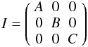 (13)with
A ≤ B ≤ C.
(13)with
A ≤ B ≤ C.
The dynamical model is a three-degree of freedom one. We used the Andoyer variables, which requires a decomposition with three references frames:
- 1.
an inertial reference frame (e1,e2,e3). We used the one in which the orbital ephemerides are given, i.e. mean Saturnian equator and mean equinox for the J2000.0 epoch;
- 2.
a frame (n1,n2,n3) bound to the angular momentum of Mimas;
- 3.
a frame (f1,f2,f3) rigidly linked to Mimas.
The canonical set of Andoyer’s variables consists of the three angular variables
l,g,h and their conjugated momenta L,G,H defined by
the norm G of the angular momentum and two of its projections:
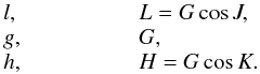 (14)Unfortunately,
these variables present two singularities: when J = 0 (i.e., the angular
momentum is colinear to f3),
l and g are undefined, and when K = 0
(i.e., when Mimas’ principal axis of inertia is perpendicular to its orbital plane),
h and g are undefined. That is the reason why we used
the modified Andoyer’s variables:
(14)Unfortunately,
these variables present two singularities: when J = 0 (i.e., the angular
momentum is colinear to f3),
l and g are undefined, and when K = 0
(i.e., when Mimas’ principal axis of inertia is perpendicular to its orbital plane),
h and g are undefined. That is the reason why we used
the modified Andoyer’s variables: ![\begin{equation} \begin{array}{lll} p=l+g+h, & \hspace{1cm} & P=\frac{G}{nC}, \\[2mm] r=-h, & \hspace{1cm} & \mathcal{R}=\frac{G-H}{nC}=P(1-\cos K), \\[2mm] & \hspace{1cm} & \phantom{\mathcal{R}}=2P\sin^2\frac{K}{2}, \\[2mm] \xi_q=\sqrt{\frac{2Q}{nC}}\sin q, & \hspace{1cm} & \eta_q=\sqrt{\frac{2Q}{nC}}\cos q, \label{equ:modified} \end{array} \end{equation}](/articles/aa/full_html/2011/12/aa17558-11/aa17558-11-eq239.png) (15)where
n is the body’s mean orbital motion,
q = −l, and
(15)where
n is the body’s mean orbital motion,
q = −l, and  .
With these new variables, the singularity on l has been dropped. Using
these variables has a great mathematical interest, because they are canonical, so they
simplify an analytical study of the system, as was done in the previous works mentioned
above. Our study here is essentially numerical, but we keep these variables to be
consistent with previous studies. We derive other output variables below, that are more
relevant from a physical point of view.
.
With these new variables, the singularity on l has been dropped. Using
these variables has a great mathematical interest, because they are canonical, so they
simplify an analytical study of the system, as was done in the previous works mentioned
above. Our study here is essentially numerical, but we keep these variables to be
consistent with previous studies. We derive other output variables below, that are more
relevant from a physical point of view.
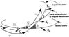 |
Fig. 2 The Andoyer variables (partially reproduced from Henrard 2005a). |
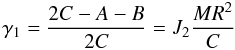
In these variables, the kinetic energy  of the system reads
![\begin{eqnarray} \label{equ:kinrj} T & = & \frac{nP^2}{2}+\frac{n}{8}\left[4P-\xi_q^2-\eta_q^2\right] \nonumber \\ && \times \left[\frac{\gamma_1+\gamma_2}{1-\gamma_1-\gamma_2}\xi_q^2+\frac{\gamma_1-\gamma_2}{1-\gamma_1+\gamma_2}\eta_q^2\right] \end{eqnarray}](/articles/aa/full_html/2011/12/aa17558-11/aa17558-11-eq243.png) (16)with
(16)with
 (17)and
 (18)In these last three
formulae, ω is the instantaneous vector of rotation,
M is the mass of Mimas, R its mean radius, and
J2 and C22 the two classical
normalized gravitational coefficients related to the oblateness and equatorial ellipticity
of the considered body, respectively.
(18)In these last three
formulae, ω is the instantaneous vector of rotation,
M is the mass of Mimas, R its mean radius, and
J2 and C22 the two classical
normalized gravitational coefficients related to the oblateness and equatorial ellipticity
of the considered body, respectively.
The gravitational disturbing potential caused by an oblate perturber p
reads (Henrard 2005c)  (19)with
![\begin{equation} V_{p1}=-\frac{3}{2}C\frac{\mathcal{G}M_{\rm p}}{d_{\rm p}^3}\left[\gamma_1\left(x_{\rm p}^2+y_{\rm p}^2\right)+\gamma_2\left(x_{\rm p}^2-y_{\rm p}^2\right)\right] \label{equ:Vpert1} \end{equation}](/articles/aa/full_html/2011/12/aa17558-11/aa17558-11-eq250.png) (20)and
(20)and
![\begin{eqnarray} V_{p2} & = & -\frac{15}{4}CJ_{2p}\frac{\mathcal{G}M_{\rm p}}{d_{\rm p}^3}\left(\frac{R_{\rm p}}{d_{\rm p}}\right)^2 \nonumber \\ && \times \left[\gamma_1\left(x_{\rm p}^2+y_{\rm p}^2\right)+\gamma_2\left(x_{\rm p}^2-y_{\rm p}^2\right)\right], \label{equ:Vpert2} \end{eqnarray}](/articles/aa/full_html/2011/12/aa17558-11/aa17558-11-eq251.png) (21)where
(21)where
 is the gravitational constant, Mp the mass of the perturber,
J2p its J2,
Rp its mean radius, dp the
distance between the perturber’s and Mimas’ centers of mass, and
xp and yp the two first
components of the unit vector pointing to the center of mass of the perturber, from the
center of mass of the body, in the reference frame
(f1,f2,f3).
Vp1 expresses the perturbation caused by a
pointmass perturber, while Vp2 represents the
perturbation caused by its J2, assuming that the body is in
the equatorial plane of the perturber. As shown in (Henrard 2005c), it is a good approximation if the sine of the angle between
Saturn’s equatorial plane and the orbit is small. In the case of Mimas, this angle (i.e.
Mimas’ orbital inclination) is ≈ 1.5° ≈ 2.6 × 10⁻² rad, so we can consider
that its sine is always smaller than 3 × 10⁻². This assertion also assumes that
the obliquity of Mimas is very low, which we will check in this study.
is the gravitational constant, Mp the mass of the perturber,
J2p its J2,
Rp its mean radius, dp the
distance between the perturber’s and Mimas’ centers of mass, and
xp and yp the two first
components of the unit vector pointing to the center of mass of the perturber, from the
center of mass of the body, in the reference frame
(f1,f2,f3).
Vp1 expresses the perturbation caused by a
pointmass perturber, while Vp2 represents the
perturbation caused by its J2, assuming that the body is in
the equatorial plane of the perturber. As shown in (Henrard 2005c), it is a good approximation if the sine of the angle between
Saturn’s equatorial plane and the orbit is small. In the case of Mimas, this angle (i.e.
Mimas’ orbital inclination) is ≈ 1.5° ≈ 2.6 × 10⁻² rad, so we can consider
that its sine is always smaller than 3 × 10⁻². This assertion also assumes that
the obliquity of Mimas is very low, which we will check in this study.
Usually the orbital ephemerides give us the location of the perturber in the inertial
frame, therefore we have to perform five rotations to convert the coordinates from the
inertial frame to
(f1,f2,f3).
More precisely, if we name
(xi,yi,zi)T
the unit vector locating the perturber’s center of mass in the inertial frame, we have
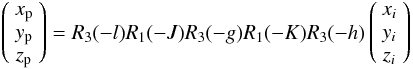 (22)with
 (23)and
 (24)Finally, the total
Hamiltonian of the problem reads
(24)Finally, the total
Hamiltonian of the problem reads ![\begin{eqnarray} H & = & \frac{nP^2}{2}+\frac{n}{8}\left[4P-\xi_q^2-\eta_q^2\right] \nonumber \\ & & \times\left[\frac{\gamma_1+\gamma_2}{1-\gamma_1-\gamma_2}\xi_q^2+\frac{\gamma_1-\gamma_2}{1-\gamma_1+\gamma_2}\eta_q^2\right] \nonumber \\ & & -\frac{3}{2n}\frac{\mathcal{G}M_{\protect\saturn}}{d_{\protect\saturn}^3}\left(1+\frac{5}{2}J_{2{}}\left(\frac{R_{\protect\saturn}}{d_{\protect\saturn}}\right)^2\right) \nonumber \\ & & \times \left[\gamma_1\left(x_{\protect\saturn}^2+y_{\protect\saturn}^2\right)+\gamma_2\left(x_{\protect\saturn}^2-y_{\protect\saturn}^2\right)\right], \label{equ:Htotal} \end{eqnarray}](/articles/aa/full_html/2011/12/aa17558-11/aa17558-11-eq267.png) (25)where
the index ♄ stands for Saturn. We will use this Hamiltonian for a numerical study of the
rotation. An analytical study can show that the Hamiltonian (25) can be reduced to
(25)where
the index ♄ stands for Saturn. We will use this Hamiltonian for a numerical study of the
rotation. An analytical study can show that the Hamiltonian (25) can be reduced to  (26)where
 represents a perturbation, and the three constants
ωu,
ωv and
ωw are the periods of the free
oscillations around the equilibrium defined by the Cassini laws. This
last Hamiltonian is obtained after several canonical transformations, the first one
consisting of expressing the resonant arguments
σ = p − λ + π and
ρ = r + ☊ respectively associated with the
1:1 spin-orbit resonance and with the orientation of the angular momentum,
λ and ☊ being the orbital variables defined above. The complete
calculation is beyond the scope of this paper, the reader can find details in Henrard (2005a,b), and Noyelles et al. (2008).
represents a perturbation, and the three constants
ωu,
ωv and
ωw are the periods of the free
oscillations around the equilibrium defined by the Cassini laws. This
last Hamiltonian is obtained after several canonical transformations, the first one
consisting of expressing the resonant arguments
σ = p − λ + π and
ρ = r + ☊ respectively associated with the
1:1 spin-orbit resonance and with the orientation of the angular momentum,
λ and ☊ being the orbital variables defined above. The complete
calculation is beyond the scope of this paper, the reader can find details in Henrard (2005a,b), and Noyelles et al. (2008).
3.3. A numerical study
To integrate the system numerically, we first express the coordinates of the perturber
(x♄,y♄) with the numerical
ephemerides and the rotations given in Eq. (22) in the body frame
(f1,f2,f3).
As explained above, the ephemerides are given by the TASS1.6 ephemerides (Vienne & Duriez 1995). This way, we obtain
coordinates depending of the canonical variables. Then we derive the equations coming from
the Hamiltonian (25) ![\begin{eqnarray} \frac{{\rm d}p}{{\rm d}t} = \frac{\partial H}{\partial P}, & & \frac{{\rm d}P}{{\rm d}t} = -\frac{\partial H}{\partial p}, \nonumber \\[1.5mm] \frac{{\rm d}r}{{\rm d}t} = \frac{\partial H}{\partial R}, & & \frac{{\rm d}R}{{\rm d}t}=-\frac{\partial H}{\partial r}, \nonumber \\[1.5mm] \frac{{\rm d}\xi_q}{{\rm d}t} = \frac{\partial H}{\partial \eta_q}, & & \frac{{\rm d}\eta_q}{{\rm d}t}=-\frac{\partial H}{\partial \xi_q}\cdot \label{equ:equhamil} \end{eqnarray}](/articles/aa/full_html/2011/12/aa17558-11/aa17558-11-eq278.png) (27)We
integrated over 200 years using the Adams-Bashforth-Moulton 10th order predictor-corrector
integrator. The solutions consist of two parts, the forced one, directly caused by the
perturbation, and the free one, which depends on the initial conditions. The initial
conditions should be as close as possible to the exact equilibrium, which is assumed to be
the Cassini state 1 in 1:1 spin-orbit resonance, to have low amplitudes
of the free librations. For that, we used the iterative algorithm NAFFO (Noyelles et al. 2011) to remove the free librations
from the initial conditions after they were identified by frequency analysis.
(27)We
integrated over 200 years using the Adams-Bashforth-Moulton 10th order predictor-corrector
integrator. The solutions consist of two parts, the forced one, directly caused by the
perturbation, and the free one, which depends on the initial conditions. The initial
conditions should be as close as possible to the exact equilibrium, which is assumed to be
the Cassini state 1 in 1:1 spin-orbit resonance, to have low amplitudes
of the free librations. For that, we used the iterative algorithm NAFFO (Noyelles et al. 2011) to remove the free librations
from the initial conditions after they were identified by frequency analysis.
The frequency analysis algorithm we used is based on Laskar’s original idea, named NAFF
for numerical analysis of the fundamental frequencies (see for instance Laskar (1993) for the method, and Laskar (2005) for the convergence proofs). It aims at identifying the
coefficients ak and
ωk of a complex signal
f(t) obtained numerically over a finite time span
[ − T;T] and verifying 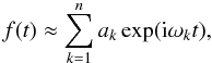 (28)where
ωk are real frequencies and
ak complex coefficients. If the signal
f(t) is real, its frequency spectrum is symmetric and
the complex amplitudes associated with the frequencies
ωk
and − ωk are complex conjugates. The
frequencies and amplitudes associated are found with an iterative scheme. To determine the
first frequency ω1, one searches for the maximum of the
amplitude of
(28)where
ωk are real frequencies and
ak complex coefficients. If the signal
f(t) is real, its frequency spectrum is symmetric and
the complex amplitudes associated with the frequencies
ωk
and − ωk are complex conjugates. The
frequencies and amplitudes associated are found with an iterative scheme. To determine the
first frequency ω1, one searches for the maximum of the
amplitude of 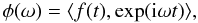 (29)where the scalar
product
⟨ f(t),g(t) ⟩ is
defined by
(29)where the scalar
product
⟨ f(t),g(t) ⟩ is
defined by 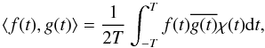 (30)and where
χ(t) is a weight function, i.e. a positive function
with
(30)and where
χ(t) is a weight function, i.e. a positive function
with 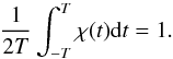 (31)Once the first periodic
term exp(iω1t) is found, its complex
amplitude a1 is obtained by orthogonal projection, and the
process is started again on the remainder
f1(t) = f(t) − a1exp(iω1t).
The algorithm stops when two detected frequencies are too close to each other, which
alters their determinations, or when the number of detected terms reaches a maximum set by
the user. This algorithm is very efficient, except when two frequencies are too close to
each other. In that case, the algorithm is not confident in its accuracy and stops. When
the difference between two frequencies is larger than twice the frequency associated with
the length of the total time interval, the determination of each fundamental frequency is
not perturbed by the other ones. Although the iterative method suggested by Champenois (1998) allows one to reduce this distance,
some difficulties remain when the frequencies are too close to each other.
(31)Once the first periodic
term exp(iω1t) is found, its complex
amplitude a1 is obtained by orthogonal projection, and the
process is started again on the remainder
f1(t) = f(t) − a1exp(iω1t).
The algorithm stops when two detected frequencies are too close to each other, which
alters their determinations, or when the number of detected terms reaches a maximum set by
the user. This algorithm is very efficient, except when two frequencies are too close to
each other. In that case, the algorithm is not confident in its accuracy and stops. When
the difference between two frequencies is larger than twice the frequency associated with
the length of the total time interval, the determination of each fundamental frequency is
not perturbed by the other ones. Although the iterative method suggested by Champenois (1998) allows one to reduce this distance,
some difficulties remain when the frequencies are too close to each other.
3.4. Outputs
To deliver theories of rotation that can be easily compared with observations, we chose to express our results in the following variables:
-
longitudinal librations;
-
latitudinal librations;
-
orbital obliquity ϵ (the orientation of the angular momentum of Mimas with respect to the normal to the instantaneous orbital plane);
-
motion of the rotation axis about the pole axis.
The latitudinal librations are the north-south librations of the large axis of the
considered body in the saturnocentric reference frame that follows the orbital motion of
the body. They are analogous to the tidal librations that are the east-west librations. To
obtain the tidal longitudinal librations and the latitudinal librations, we first express
the unit vector f1 (i.e. the
direction of Mimas’ long axis) in the inertial frame
(e1,e2,e3).
From (Eq. (22)) and the definitions of the
Andoyer modified variables (Eq. (15)), we obtain: 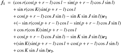 (32)The
tidal longitudinal librations ψ and the latitudinal ones
η are found by
(32)The
tidal longitudinal librations ψ and the latitudinal ones
η are found by  (33)and
 (34)where
n is the unit vector normal to the orbit plane, and
t the tangent to the trajectory. We compute these last
two vectors by
(34)where
n is the unit vector normal to the orbit plane, and
t the tangent to the trajectory. We compute these last
two vectors by  (35)and
 (36)where
x is the position vector of the body, and
v its velocity.
(36)where
x is the position vector of the body, and
v its velocity.
Finally, the motion of the rotation axis about the pole is derived from the wobble
J, it is given by the two variables Q1 and
Q2 defined as  (37)and
 (38)they are the first two
components of the unit vector pointing at the instantaneous north pole of Mimas’ rotation
axis in the body frame of Mimas. These quantities are finally multiplied by the polar
radius of the satellite, i.e. 190.6 km (Thomas
2010) to obtain a deviation in meters.
(38)they are the first two
components of the unit vector pointing at the instantaneous north pole of Mimas’ rotation
axis in the body frame of Mimas. These quantities are finally multiplied by the polar
radius of the satellite, i.e. 190.6 km (Thomas
2010) to obtain a deviation in meters.
4. Results
We here present the outputs of our numerical study of the rotation of Mimas. We first give the example of a non-hydrostatic model of Mimas based on its observed shape, then we compare the results with the rotational response of the first 22 models of Table 2, obtained considering Mimas to be in hydrostatic equilibrium.
4.1. Non-hydrostatic Mimas based on its shape
As already mentioned, this case is unique, because changes in the size of the core do not affect the ratios of the moments of inertia A/C, and B/C, and the coefficients γ1 and γ2 (Eqs. (17) and (18)). Consequently, there is a unique rotational behaviour of Mimas for any homogenous or two-layer model using this specific model based on the observed shape.
The free librations around the equilibrium are assumed to be damped, it is in any case important to know their frequencies ωu, ωv and ωw (or periods Tu, Tv and Tw) because they characterize the way the system reacts to external sinusoidal excitations, which are here caused by the variations of the distance between the Sun and Mimas.
Frequencies and periods of the free librations of Mimas in the shape model.
The frequencies of the free librations are listed in Table 4. The proper mode u roughly represents the free longitudinal librations, v the free librations of the obliquity, and w the wobble, i.e. the free polar motion of Mimas. These frequencies were deduced from the frequency analysis of the modified Andoyer variables (cf. Eq. (15)).
The proper modes involved in the Fourier representations of the librations of Mimas are the forced modes caused by the orbital motion of Mimas around Saturn (cf. Table 3) and the free ones (Table 4). The arguments of the sinusoidal components of the quasi-periodic decompositions of the rotation variables are integer combinations of these proper modes. If we consider that the free librations are damped, the solutions should be only composed of the forced modes.
Forced tidal longitudinal librations of Mimas in the shape model.
Forced physical longitudinal librations of Mimas in the shape model.
Forced latitudinal librations of Mimas in the shape model.
Forced obliquity of Mimas in the shape model.
The forced librations of Mimas modelled from its observed shape are given in Tables 5 to 8. These tables give the solutions in the form of periodic time series in cosines. Evidently, the main difference between the physical and the tidal librations is in the presence in the physical librations of a long-period term ( ≈ 70 years) with a high amplitude ( ≈ 43°, i.e. ≈ 86° peak-to-peak) caused by the librations of the argument of the orbital resonance between Mimas and Tethys. As explained in Rambaux et al. (2010, 2011), the amplitude of the long-period librations are equal to the magnitude of the orbital perturbations because at long period the body is oriented towards the central planet. As a consequence, by analysing the tidal librations, the long period librations vanish. There is also a considerable difference in the amplitude given for the tidal and physical longitudinal librations. As explained above, this difference is caused by optical librations, with amplitude 2e ≈ 3.8 × 10⁻² rad ≈ 2.2°.
The latitudinal librations of Mimas (Table 7) are significantly smaller ( ≈ 2 arcmin vs. 2.5° for the tidal longitudinal librations), and so could hardly be used in the framework of observations of the rotation of Mimas (except if there are free oscillations due to a recent unexpected excitation). The mean obliquity of Mimas (Table 8) is of the same order of magnitude.
4.2. For a hydrostatic Mimas
We performed the same numerical study for the 22 hydrostatic configurations of Mimas given in Table 2. The results are gathered in Table 9. In this table, the amplitudes of the tidal and physical longitudinal librations indicated are related to the mode λ − φ + ζ (period: 0.944898 d), while the latitudinal ones are related to the mode λ + φ − ζ (period: 0.939962 d). The main physical reason for these librations is the variation of the distance Mimas-Saturn during an orbital period.
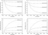 |
Fig. 3 Librations of hydrostatic Mimas depending on the densities of the core and the shell. |
Periods of the free librations and amplitudes (in arcmin) of the forced librations for the different models assuming that Mimas is in the hydrostatic equilibrium.
To make the results more readable, we present them graphically in Fig. 3. The plots present a clear dependency of the amplitudes of librations on the densities of the core and the shell. We can notice in particular that the longitudinal (i.e. tidal and physical) librations have a larger amplitude when the density of the core is lower, which is because a concentration of the mass in the core lowers the moments of inertia of the body, and so tends to limit its amplitude of response to solicitations. Finally we can see that the dependency on ρc is small for ρs = 1100 kg/m3, it is because in this case, ρs is close to the mean density of Mimas (i.e. 1150.03 kg/m3), as a consequence the core is small and Mimas is close to be homogeneous.
4.3. A small polar motion
We present the forced polar motion of Mimas (i.e. after removal of the free wobble) as a sum of a trigonometric series (Table 10). We can see that this motion is expected to be small, the highest amplitude being ≈ 15 m. The sum of all these amplitudes can reach 40 m, so we can consider these 40 m as the upper bound of the polar motion. An analysis of the polar motions for the different hydrostatic Mimas does not exhibit significant differences.
5. Tidal dissipation
Polar motion of Mimas q1 + iq2 in the shape model.
This section is dedicated to study the influence of the tidal torque on the rotational
motion of Mimas. We introduce the tidal torque in a Lagrangian formalism and follow the
approach of Williams et al. (2001) that was also recently used in Rambaux et al. (2010) and
Robutel et al. (2011). The starting equation is the angular momentum equation  (39)where
ω is the angular velocity vector, the angular momentum
G = Iω with
I the tensor of inertia, and T is the
external gravitational torque expressed as
(39)where
ω is the angular velocity vector, the angular momentum
G = Iω with
I the tensor of inertia, and T is the
external gravitational torque expressed as
 (40)where
u is the cosine director of Saturn in the reference frame
tied to Mimas, and M♄ its mass.
(40)where
u is the cosine director of Saturn in the reference frame
tied to Mimas, and M♄ its mass.
The dissipation is caused by the tidal and centrifugal potentials that deform the satellite. In this case, the tensor of inertia I becomes a constant plus a time-variable part resulting from the deformation. The time-variable part does not react instantaneously and therefore presents a time delay δt characteristics of the rheological properties of the body (see Sect. 2).
In addition, the dynamical equation of the rotational motion Eq. (39) may be linearized by using the synchronous spin-orbit resonance of the body implying that ω1,ω2 ≪ ω3 ~ n and u2,u3 ≪ u1 ~ 1 where u1,u2,u3 are the coordinates of the cosine director along the principal axis of inertia of Mimas.
By using these approximations and focusing on the libration in longitude, the main tidal
torque is expressed as (Williams et al. 2001)
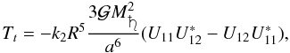 (41)where
 and the star indicates
the time-delay part.
and the star indicates
the time-delay part.
Then, we used the same approach as in Rambaux et al. (2010). We introduce the rotation
angle ϕ similar to the sum of the Andoyer angles
l + g because the polar motion is small, as shown in
Fig. 2, where J and
θ (the nutation angle) are small. The libration angle γ
is defined as ϕ = M + γ representing the
physical libration in longitude of the body. The cosine director
u2 ~ s − γ is of
the order of the difference between the orbital variation s and the
physical libration γ. We note that u2
corresponds to the tidal libration ψ defined in Sect. 3.4 and their amplitude is small as shown in Table 5. The quantity
s, the orbital variation, is defined as the difference between the true
and the mean longitude of Mimas and represents the oscillation of the orbital longitude of
Mimas that may be expressed in Fourier series as
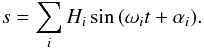 (42)Then, by developing
 and
and
 in Taylor
series for small δt, the dynamical equation becomes
in Taylor
series for small δt, the dynamical equation becomes 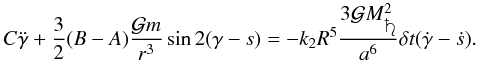 (43)As shown in the
previous section, the quantity γ − s is always small (see
Table 5) allowing us to simplify the sine function by its angle. In addition, the
eccentricity of Mimas is low and so a/r is equal to 1 at
first order in eccentricity. Finally, we obtain a forced dissipative harmonic oscillator
with the frequency
(43)As shown in the
previous section, the quantity γ − s is always small (see
Table 5) allowing us to simplify the sine function by its angle. In addition, the
eccentricity of Mimas is low and so a/r is equal to 1 at
first order in eccentricity. Finally, we obtain a forced dissipative harmonic oscillator
with the frequency  and the dissipative rate λ expressed as
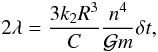 (44)m
being the mass of the satellite and k2 is the Love number of
Mimas.
(44)m
being the mass of the satellite and k2 is the Love number of
Mimas.
In the conservative case, the amplitude of terms associated with the long period is almost
equal to the magnitude of the oscillation s. The solution may be expressed
as  (45)where
Ad and
φd are constants of integration. The first
term decays with time scale 1/λ and its resonant frequency is
(45)where
Ad and
φd are constants of integration. The first
term decays with time scale 1/λ and its resonant frequency is
 .
The periodic term of the particular solution γ is composed of the in-phase
yi and out-of-phase
xi terms
.
The periodic term of the particular solution γ is composed of the in-phase
yi and out-of-phase
xi terms 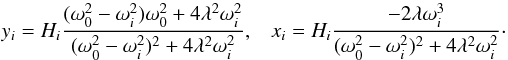 (46)At first order, the
expression of xi may be simplified as
(46)At first order, the
expression of xi may be simplified as
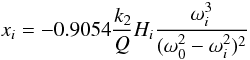 (47)expressed
in radians and by introducing the dissipation factor as
δt = (nQ)-1. For short-period librations at
0.944898 days the xi is 1.32 mas with
(47)expressed
in radians and by introducing the dissipation factor as
δt = (nQ)-1. For short-period librations at
0.944898 days the xi is 1.32 mas with
 (this is the value used by Meyer & Wisdom
2008) and the resulting displacement at the surface of the satellite at the
periaster passage is also negligible 0.0013 m. The damping time 1/λ is
about 6000 years. If we consider
(this is the value used by Meyer & Wisdom
2008) and the resulting displacement at the surface of the satellite at the
periaster passage is also negligible 0.0013 m. The damping time 1/λ is
about 6000 years. If we consider  to
be 100 times bigger, i.e. closer to the expected value of Enceladus, we have a displacement
at the surface of ≈ 0.13 m and a damping time of ≈ 60 years. For librations at long period
xi is definitely negligible because
ωi is very small.
to
be 100 times bigger, i.e. closer to the expected value of Enceladus, we have a displacement
at the surface of ≈ 0.13 m and a damping time of ≈ 60 years. For librations at long period
xi is definitely negligible because
ωi is very small.
6. Discussion
One of the aims of this theoretical study is to prepare the interpretation of potential observations of the rotation of Mimas. After a restricted analytical approach to validate the numerical results, we discuss the possibility to observe the rotation of Mimas and in particular to distinguish the different interior models. Then we focus on the non-hydrostatic contributions.
6.1. Analytical approach
We here compare with classical analytical formulae for the main term of the physical and tidal longitudinal librations and the mean obliquity, for which deriving these amplitudes accurately is quite straightforward.
6.1.1. Longitudinal librations
An analytical study of the longitudinal librations of a satellite in 1:1 spin-orbit
resonance and on a Keplerian orbit can be found for instance in Murray & Dermott (1999). Let us call ψ the
amplitude of the main term (i.e. associated with the mode
λ + φ − ζ) of the tidal librations,
and γ for the physical ones. We have from Murray & Dermott (1999)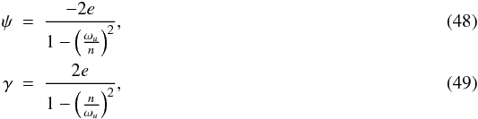 and
and
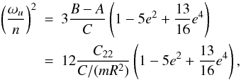 (50)e
being the eccentricity of Mimas. We can see that this amplitude is bigger when the ratio
is closer to unity, or when 12C22 is closer to
C/(mR2). We can see from
Table 2 that C22 is
of the order 5 × 10⁻³ while
C ≈ 0.4mR2, i.e.
C22/C/(mR2) ≈ 1/80.
Thus, the ratio
(50)e
being the eccentricity of Mimas. We can see that this amplitude is bigger when the ratio
is closer to unity, or when 12C22 is closer to
C/(mR2). We can see from
Table 2 that C22 is
of the order 5 × 10⁻³ while
C ≈ 0.4mR2, i.e.
C22/C/(mR2) ≈ 1/80.
Thus, the ratio  is closer to unity when C22 is bigger, which is the case for
the lowest values of ρc. Figure 3 confirms this trend, while the Table 11 settles the validity of the analytical formulae (48) and (49).
is closer to unity when C22 is bigger, which is the case for
the lowest values of ρc. Figure 3 confirms this trend, while the Table 11 settles the validity of the analytical formulae (48) and (49).
6.1.2. Mean obliquity
We here use the analytical study of Ward & Hamilton (2004; see Noyelles 2010, for an application to natural
satellites in spin-orbit resonances) for the location of the Cassini
states. Mimas is expected to be locked at the Cassini state 1,
i.e. the most stable one, characterized by  (51)ϵ
being the mean obliquity of Mimas,
(51)ϵ
being the mean obliquity of Mimas,  the precessional rate of its orbital ascending node, and I its
inclination on the Laplace plane, here assumed to be the equator of Saturn at J2000.
the precessional rate of its orbital ascending node, and I its
inclination on the Laplace plane, here assumed to be the equator of Saturn at J2000.
From the definition the orbital proper modes of Mimas, we can approximate
by  rad/y, this yields a regressional period of 360.1657 days. In assuming
J2 ≈ 2 × 10⁻²,
C22 ≈ 6 × 10⁻³ and
C ≈ 0.4mR2 from
Table 2, we have
rad/y, this yields a regressional period of 360.1657 days. In assuming
J2 ≈ 2 × 10⁻²,
C22 ≈ 6 × 10⁻³ and
C ≈ 0.4mR2 from
Table 2, we have
 while
sinI is very small and cosI close to unity (the mean
inclination of Mimas I being of the order of
1.5° = 2.6 × 10⁻² rad). This means that higher values of the quantity
J2 + 2C22 will yield a lower
obliquity. Once more, these values are reached for the lowest estimations of
ρc, Fig. 3 confirming
this tendency. The validity of the analytical formula (51) is checked in Table 11.
while
sinI is very small and cosI close to unity (the mean
inclination of Mimas I being of the order of
1.5° = 2.6 × 10⁻² rad). This means that higher values of the quantity
J2 + 2C22 will yield a lower
obliquity. Once more, these values are reached for the lowest estimations of
ρc, Fig. 3 confirming
this tendency. The validity of the analytical formula (51) is checked in Table 11.
The remaining question for analytical validation is: how does one evaluate the mean eccentricity and inclination required in the analytical formulae, i.e. how does one average them? These formulae were derived in assuming a Keplerian orbit, while the orbit of Mimas is perturbed by the oblateness of Saturn and the mutual interactions with the other satellites, inducing an orbital resonance with Tethys. As a consequence, its eccentricity and inclination are far from constant.
We have from Vienne & Duriez
(1995)![\begin{eqnarray} z(t) & = & e(t)\exp\left({\rm i}\varpi(t)\right) \nonumber \\[1.5mm] & = & 1.59817\times10^{-2}\exp\left({\rm i}\left(6.38121472t+356.521^{\circ}\right)\right) \nonumber \\[1.5mm] && + 7.2147\times10^{-3}\exp\left({\rm i}\left(6.29216934t+137.197^{\circ}\right)\right) \label{eq:ztass} \\[1.5mm] && + 7.1114\!\times\!10^{-3}\exp\left({\rm i}\left(6.47026010t\!+\!35.846^{\circ}\right)\right)\!+\ldots, \nonumber \\[3.5mm] \zeta(t) & = & \sin\left(\frac{I(t)}{2}\right)\left({\rm i}\ascnode(t)\right) \nonumber \\[1.5mm] & = & 1.18896\times10^{-2}\exp\left({\rm i}\left(-6.37188169t+234.213^{\circ}\right)\right) \nonumber \\[1.5mm] & &+ 5.3177\times10^{-3}\exp\left({\rm i}\left(-6.46092707t+14.888^{\circ}\right)\right) \label{eq:zetatass} \\[1.5mm] & &+ 5.3017\!\times\!10^{-3}\exp\left({\rm i}\left(-6.28283631t\!+\!273.538^{\circ}\right)\right)\!+\ldots, \nonumber \end{eqnarray}](/articles/aa/full_html/2011/12/aa17558-11/aa17558-11-eq655.png) the
frequencies are given in rad/year, and the time origin J1980. Evidently, the mean
eccentricity should be at least ≈ 1.6 × 10⁻², probably higher (same for the
mean inclination, which should be at least ≈ 1.4°). In Table 11 we use e = 1.92 × 10⁻² and
I = 1.68°, this arbitrary choice minimizes the relative errors and is
consistent with the TASS1.6 theory.
the
frequencies are given in rad/year, and the time origin J1980. Evidently, the mean
eccentricity should be at least ≈ 1.6 × 10⁻², probably higher (same for the
mean inclination, which should be at least ≈ 1.4°). In Table 11 we use e = 1.92 × 10⁻² and
I = 1.68°, this arbitrary choice minimizes the relative errors and is
consistent with the TASS1.6 theory.
6.2. Observational possibilities
It would be challenging to constrain the orientation and interior structure of Mimas using its rotation. The first expected result is the confirmation that Mimas is in the Cassini state 1 with the 1:1 spin-orbit resonance. Another challenge would be to detect the longitudinal librations, which have been actually observed for the Moon (Koziel 1967), the Martian satellite Phobos (Burns 1972), and the Saturnian satellite Epimetheus (Tiscareno et al. 2009). To estimate the required accuracy of the observations, we convert the rotation outputs into kilometres (Table 12).
Expected librations and mean obliquity of Mimas in km.
As expected, the longitudinal librations are significantly bigger (a few kilometres) than the mean obliquity and the latitudinal librations (with an amplitude smaller than 200 m). The amplitude of the librations given are related to the quasi-periodic decompositions, so the peak-to-peak amplitudes are twice as big. The reader should keep in mind that the physical and tidal librations are two expressions of the same quantity, so are not independent. We can consider that the detection of the longitudinal librations would require an accuracy of about 1 km, while using them to invert the internal structure of Mimas would require an accuracy at least ten times better.
6.3. Non-hydrostatic contributions
The study of the non-hydrostatic Mimas based on the shape model does not exhibit a significant possibility to distinguish a non-hydrostatic Mimas from a hydrostatic one from observations. This is not surprising considering Mimas’ nearly hydrostatic global shape. But a non-hydrostatic Mimas could result in an offset between the ellipsoid of shape and the ellipsoid of inertia, as investigated for Janus by Robutel et al. (2011), for which an offset in longitude and in latitude has actually been detected (Tiscareno et al. 2009). Consequently, detection of non-hydrostatic contributions from observation of Mimas’ orientation should not a priori be excluded.
7. Conclusion
We have presented a theoretical study of the rotation of Mimas considering the three degrees of freedom of the rigid rotation, and different possible interior models, assuming Mimas to be in hydrostatic equilibrium, or not. Moreover, we considered a complete orbital motion, and also investigated the influence of tides on the rotation of Mimas.
We estimated the physical longitudinal librations to have an amplitude of about 0.5°, i.e. nearly 2 km, the exact value depending on the internal structure of Mimas. For a hydrostatic Mimas, a dense core lowers this amplitude. Non-hydrostatic contributions were shown to be small, as expected from Mimas’ shape in near hydrostatic equilibrium. Moreover, we expect an obliquity between 2 and 3 arcmin, while the polar motion can be neglected. The tidal deviation of Mimas’ long axis should be negligible as well, while this is the most inner main Saturnian satellite.
The Cassini spacecraft has already completed its initial four-year mission and the first extended mission, with a limited number of Mimas flybys. Its orbit close to Saturn makes Mimas a difficult target for Cassini observations. Since September 2010 Cassini is in a second extended mission called the Cassini Solstice Mission during (and especially at the end) of which Cassini will likely have additional Mimas observations. We hope that future observations of Mimas will allow us to constrain its rotation and to obtain clues on its internal structure and orientation.
Acknowledgments
Numerical simulations were made on the local computing ressources (Cluster URBM-SYSDYN) at the University of Namur. This work has been supported by EMERGENCE-UPMC grant (contract number: EME0911).
References
- Allan, R. R. 1969, AJ, 74, 497 [NASA ADS] [CrossRef] [Google Scholar]
- Andoyer, H. 1926, Mécanique céleste (Paris: Gauthier-Villars) [Google Scholar]
- Arnold, V. I. 1963, Uspekhi Mat. Nauk., 18, 13, in Russian. English translation: Russian Mathematical Surveys, 18, 9 [Google Scholar]
- Burns, J. A. 1972, Rev. Geophys. Space Phys., 10, 463 [NASA ADS] [CrossRef] [Google Scholar]
- Cassini, G. D. 1693, Traité de l’origine et du progrès de l’astronomie, Paris [Google Scholar]
- Champenois, S. 1998, Dynamique de la résonance entre Mimas et Téthys, premier et troisième satellites de Saturne, Ph.D. Thesis, Observatoire de Paris [Google Scholar]
- Champenois, S., & Vienne, A. 1999a, Icarus, 140, 106 [NASA ADS] [CrossRef] [Google Scholar]
- Champenois, S., & Vienne, A. 1999b, Cel. Mech. Dyn. Astr., 74, 111 [Google Scholar]
- Colombo, G. 1966, AJ, 71, 891 [NASA ADS] [CrossRef] [Google Scholar]
- Comstock, R. L., & Bills, B. G. 2003, J. Geophys. Res., 108, 5100 [NASA ADS] [CrossRef] [Google Scholar]
- Deprit, A. 1967, Am. J. Phys., 35, 424 [NASA ADS] [CrossRef] [Google Scholar]
- Dermott, S. F., & Thomas, P. C. 1988, Icarus, 73, 25 [NASA ADS] [CrossRef] [Google Scholar]
- Eluszkiewicz, J. 1990, Icarus, 84, 215 [NASA ADS] [CrossRef] [Google Scholar]
- Henrard, J. 2005a, Icarus, 178, 144 [NASA ADS] [CrossRef] [Google Scholar]
- Henrard, J. 2005b, Cel. Mech. Dyn. Astr., 91, 131 [NASA ADS] [CrossRef] [Google Scholar]
- Henrard, J. 2005c, Cel. Mech. Dyn. Astr., 93, 101 [NASA ADS] [CrossRef] [Google Scholar]
- Howett, C. J. A., Spencer, J. R., Schenk, P., et al. 2011, Icarus, in press [Google Scholar]
- Hubbard, W. B., & Anderson, J. D. 1978, Icarus, 33, 336 [NASA ADS] [CrossRef] [Google Scholar]
- Jacobson, R. A., Antreasian, P. G., Bordi, J. J., et al. 2006, AJ, 132, 2520 [NASA ADS] [CrossRef] [Google Scholar]
- Johnson, T. V., Castillo-Rogez, J., & Matson, D. L. 2006, DPS meeting 38, 69.03, BAAS, 38, 621 [NASA ADS] [Google Scholar]
- Koziel, K. 1967, Icarus, 7, 1 [NASA ADS] [CrossRef] [Google Scholar]
- Lambeck, K., & Pullan, S. 1980, Phys. Earth Planet. Interiors, 22, 29 [NASA ADS] [CrossRef] [Google Scholar]
- Laskar, J. 1993, Cel. Mech. Dyn. Astr., 56, 191 [Google Scholar]
- Laskar, J. 2005, Frequency map analysis and quasiperiodic decomposition, in Hamiltonian systems and fourier analysis: new prospects for gravitational dynamics, ed. Benest et al., Cambridge Sci. Publ., 99 [Google Scholar]
- Meyer, J., & Wisdom, J. 2008, Icarus, 193, 213 [NASA ADS] [CrossRef] [Google Scholar]
- Moser, J. 1962, Nachr. Akad. Wiss. Göttingen, Math. Phys., 2, 1 [NASA ADS] [Google Scholar]
- Munk, W. H., & MacDonald, G. J. 1960, The rotation of the Earth: A geophysical discussion (Cambridge: Cambridge University Press) [Google Scholar]
- Murray, C. D., & Dermott, S. F. 1999, Solar System Dynamics (Cambridge: Cambridge University Press) [Google Scholar]
- Nekhoroshev, N. N. 1977, Russian Mathematical Surveys, 32, 1 [Google Scholar]
- Nekhoroshev, N. N. 1979, Trudy Sem., Petrovs., 5, 5 [Google Scholar]
- Noyelles, B. 2010, Icarus, 207, 887 [NASA ADS] [CrossRef] [Google Scholar]
- Noyelles, B., Lemaitre, A., & Vienne, A. 2008, A&A, 478, 959 [NASA ADS] [CrossRef] [EDP Sciences] [Google Scholar]
- Noyelles, B., Delsate, N., & Carletti, T. 2011, Physica D, submitted [arXiv:1101.2138] [Google Scholar]
- Rambaux, N., Castillo-Rogez, J. C., Williams, J. G., & Karatekin, Ö. 2010, Geophys. Res. Lett., 37, L04202 [NASA ADS] [CrossRef] [Google Scholar]
- Rambaux, N., Van Hoolst, T., & Karatekin, Ö. 2011, A&A, 527, A118 [NASA ADS] [CrossRef] [EDP Sciences] [Google Scholar]
- Rappaport, N., Bertotti, B., Giamperi, G., & Anderson, J. D. 1997, Icarus, 126, 313 [NASA ADS] [CrossRef] [Google Scholar]
- Roatsch, Th., Wählisch, M., Hoffmeister, A., et al. 2009, Planet. Space Sci., 57, 83 [NASA ADS] [CrossRef] [Google Scholar]
- Robutel, P., Rambaux, N., & Castillo-Rogez, J. C. 2011, Icarus, 211, 758 [NASA ADS] [CrossRef] [Google Scholar]
- Struve, H. 1891, MNRAS, 51, 251 [NASA ADS] [Google Scholar]
- Thomas, P. C. 2010, Icarus, 208, 395 [NASA ADS] [CrossRef] [Google Scholar]
- Thomas, P. C., Burns, J. A., Helfenstein, P., et al. 2007, Icarus, 190, 573 [NASA ADS] [CrossRef] [Google Scholar]
- Tiscareno, M. S., Thomas, P. C., & Burns, J. A. 2009, Icarus, 204, 254 [NASA ADS] [CrossRef] [Google Scholar]
- Vienne, A., & Duriez, L. 1995, A&A, 297, 588 [NASA ADS] [Google Scholar]
- Ward, W. R., & Hamilton, D. P. 2004, AJ, 128, 2501 [NASA ADS] [CrossRef] [Google Scholar]
- Yasui, M., & Arakawa, M. 2009, J. Geophys. Res., 114, E09004 [NASA ADS] [CrossRef] [Google Scholar]
- Zebker, H. A., Stiles, B., Hensley, S., et al. 2009, Science, 324, 921 [NASA ADS] [CrossRef] [Google Scholar]
Appendix A: Notations used in the paper
Notations used in the paper.
All Tables
The proper frequencies of Mimas’ orbital motion (from TASS1.6, Vienne & Duriez 1995).
Periods of the free librations and amplitudes (in arcmin) of the forced librations for the different models assuming that Mimas is in the hydrostatic equilibrium.
All Figures
|
Fig. 1 Variations of the moment of inertia factor (MOI) with icy shell and rocky core densities. |
| In the text | |
|
Fig. 2 The Andoyer variables (partially reproduced from Henrard 2005a). |
| In the text | |
|
Fig. 3 Librations of hydrostatic Mimas depending on the densities of the core and the shell. |
| In the text | |
Current usage metrics show cumulative count of Article Views (full-text article views including HTML views, PDF and ePub downloads, according to the available data) and Abstracts Views on Vision4Press platform.
Data correspond to usage on the plateform after 2015. The current usage metrics is available 48-96 hours after online publication and is updated daily on week days.
Initial download of the metrics may take a while.