| Issue |
A&A
Volume 525, January 2011
|
|
|---|---|---|
| Article Number | A90 | |
| Number of page(s) | 15 | |
| Section | Galactic structure, stellar clusters and populations | |
| DOI | https://doi.org/10.1051/0004-6361/201014840 | |
| Published online | 03 December 2010 | |
Probing the Galactic thick disc vertical properties and interfaces⋆,⋆⋆
1
GEPI, Observatoire de Paris, CNRS, Université Paris Diderot,
5 place Jules Janssen,
92190
Meudon,
France
e-mail: This email address is being protected from spambots. You need JavaScript enabled to view it.
2
Laboratoire d’Astrophysique de Bordeaux, CNRS - Université
Bordeaux 1, 2 rue de l’Observatoire, BP 89, 33271
Floirac Cedex,
France
e-mail: This email address is being protected from spambots. You need JavaScript enabled to view it.
3
GEPI, Observatoire de Paris, CNRS, Université Paris Diderot,
61 avenue de l’Observatoire, 75014
Paris,
France
e-mail: This email address is being protected from spambots. You need JavaScript enabled to view it.
4
Universidade de São Paulo, IAG, Rua do Matão 1226, 05508-900
São Paulo,
Brazil
e-mail: This email address is being protected from spambots. You need JavaScript enabled to view it.
5
Boston University, 725 Commonwealth Ave, Boston, MA
02215,
USA
e-mail: This email address is being protected from spambots. You need JavaScript enabled to view it.
6
Observatoire de Strasbourg 11,
rue de l’Université,
67000
Strasbourg,
France
e-mail: This email address is being protected from spambots. You need JavaScript enabled to view it.
Received: 21 April 2010
Accepted: 13 September 2010
Abstract
Aims. This work investigates the properties (metallicity and kinematics) and interfaces of the Galactic thick disc as a function of height above the Galactic plane. The main aim is to study the thick disc in a place where it is the main component of the sample.
Methods. We take advantage of former astrometric work in two fields of several square degrees in which accurate proper motions were measured down to V-magnitudes of 18.5 in two directions, one near the north galactic pole and the other at a galactic latitude of 46° and galactic longitude near 0°. Spectroscopic observations have been acquired in these two fields for a total of about 400 stars down to magnitude 18.0, at spectral resolutions of 3.5 to 6.25 Å. The spectra have been analysed with the code ETOILE, comparing the target stellar spectra with a grid of 1400 reference stellar spectra. This comparison allowed us to derive the parameters effective temperature, gravity, [Fe/H] and absolute magnitude for each target star.
Results. The Metallicity Distribution Function (MDF) of the thin-thick-disc-halo system is derived for several height intervals between 0 and 5 kpc above the Galactic plane. The MDFs show a decrease of the ratio of the thin to thick disc stars between the first and second kilo-parsec. This is consistent with the classical modelling of the vertical density profile of the disc with 2 populations with different scale heights. A vertical metallicity gradient, ∂ [Fe/H] /∂z = −0.068 ± 0.009 dex kpc-1, is observed in the thick disc. It is discussed in terms of scenarios of formation of the thick disc.
Key words: Galaxy: disk / stars: abundances / Galaxy: abundances
Based on observations obtained at the Canada-France-Hawaii Telescope (CFHT) which is operated by the National Research Council of Canada, the Institut National des Sciences de l’Univers of the Centre National de la Recherche Scientifique of France, and the University of Hawaii and at the T193cm telescope, Observatoire de Haute-Provence, France.
Full Tables A.1–A.3, B.1–B.3 are only available in electronic form at the CDS via anonymous ftp to cdsarc.u-strasbg.fr (130.79.128.5) or via http://cdsarc.u-strasbg.fr/viz-bin/qcat?J/A+A/525/A90
© ESO, 2010
1. Introduction
The determination of the properties of the thick disc of the Milky Way has been a longstanding issue since its detection nearly three decades ago (Gilmore & Reid 1983). However, its formation and more generally the formation and evolution of the whole galactic disc, is not yet fully understood. Several models are proposed for the formation of the thick disc: direct accretion of material, stars and/or gas, in merger(s) (Abadi et al. 2003), accretion of gas-rich building blocks (Brook et al. 2005), the violent dynamical heating of a pre-existing disc by merger(s)1 (Quinn et al. 1993; Read et al. 2008; Kazantzidis et al. 2008; Villalobos & Helmi 2008), dynamical heating by merger(s) followed by the perturbations induced by the “re-growth” of a thin disc (Villalobos et al. 2010), the dissipational collapse of gas (Jones & Wyse 1983; Burkert et al. 1992), or the dynamical heating and radial mixing by spiral arms and molecular clouds (Schönrich & Binney 2009a,b).
Each scenario is supposed to imprint typical signatures into the velocity and metallicity distributions of the stars which were formed during these events. For this reason there have been numerous studies devoted to the determination of the thick disc velocity ellipsoid and metallicity distribution, the study of the thin disc to the thick disc interface, abundance trends and correlations between abundance and kinematics, or existence of gradients. However, the properties of the thick disc are not yet well established due to several problems like the limited amount of high resolution spectroscopic data for distant stars, biases in local samples, or the complexity of deconvolving the thick disc from the halo and the thin disc. Nonetheless, many studies aim to improve the understanding of the properties, origin and history of the thick disc.
On the one hand, high resolution, high signal to noise spectra have been obtained in the solar neighbourhood: Fuhrmann (1998, 2004, 2008), Prochaska et al. (2000), Mishenina et al. (2004), Soubiran & Girard (2005), Reddy et al. (2006), Feltzing et al. (2003), Bensby et al. (2003, 2004, 2005, 2007), Meléndez et al. (2008), Alves-Brito et al. (2010). These studies provide detailed information on the chemical composition of the thin and thick disc stars in the local volume (i.e. several hundred parsecs around the Sun). In particular, they all show that thick disc stars are enriched in alpha-elements with respect to thin disc stars. These studies also face difficulties. The thick disc is poorly represented there as it constitutes only a few to about 10% of the old thin disc. Reylé & Robin (2001) found a thick-to-thin disc proportion of 6.2%, while Siegel et al. (2002), who give a review of the thick disc local density/scale height determinations, find 6 to 10% after correcting for a variety of observational and selection biases. The Hercules stream, which is believed to have a purely dynamical origin (Famaey et al. 2005), has kinematical properties which overlap those of the thin and thick disc, complicating their deconvolution. These studies probe the local volume and therefore have a limited view of the large scale structure of the thick disc, e.g. radial, azimuthal and vertical structure or possible gradients.
On the other hand, photometric and low/intermediate resolution spectroscopic surveys and studies are investigating the large scale (i.e. several kilo-parsecs) properties of the Galactic populations and their interfaces: the Sloan Digital Sky Survey, SDSS (Abazajian et al. 2003, 2009; Allende Prieto et al. 2006; Ivezić et al. 2008; Bond et al. 2010; Carollo et al. 2010), synthesis of photometric observations (Reylé & Robin 2001), photometry in Kapteyn Selected Areas (Siegel et al. 2002, 2009), the Radial Velocity Experiment, RAVE (Steinmetz et al. 2006; Zwitter et al. 2008; Veltz et al. 2008), the Sloan Extension for Galactic Understanding and Exploration, SEGUE (Yanny et al. 2009). Some results of these studies are discussed in Sect. 4.3.
Our survey belongs to the second category: i.e. low resolution spectroscopy of stars probing several kilo-parsecs above the Galactic plane. Of course, the statistics of our sample is much more modest than the ones of the large surveys cited above. It contains about 400 stars and probes two canonical directions up to several kilo-parsecs above the Galactic plane. We have obtained low resolution spectra of Δλ = 3.5 Å and 6.25 Å for stars down to V = 18 also having good proper motions available. From these spectra we have obtained atmospheric parameters, as well as radial velocities for the higher resolution sample. The two fields studied are near the North Galactic Pole (NGP), l = 51°, b = 80°, and at intermediate galactic latitude pointing “above” the bulge (l = 5°, b = 46°) where proper motions surveys were conducted by Soubiran (1992) and Ojha et al. (1994), respectively.
The analysis of a large dataset of spectra implies the use of automated methods for the determination of atmospheric parameters. The originality of our approach, based on a minimum distance criterion, is the use of a large library of observed spectra to estimate the absolute magnitude of the target stars simultaneously and on the same principle as the atmospheric parameters. As a consequence we obtain distances for our target stars with a precision of the order of 30%. We have taken care to build a high quality reference library with stars having published atmospheric parameters relying on high quality data and with Hipparcos stars with accurate distances as good references for the absolute magnitudes.
Sect. 2 describes the observations. Sect. 3 presents the ETOILE code which was developed in order to obtain radial velocities, atmospheric parameters (Teff, log g, [Fe/H]) and absolute magnitudes MV. In Sect. 4 the data at large distances from the galactic plane are analysed. The results are summarised in Sect. 5.
2. The observations
We performed observations of field stars in two galactic directions, nearby the globular clusters M 3 and M 5, but sufficiently far away to avoid the contamination of the observed samples by stars belonging to the clusters. The first field, hereafter FM3 field, is nearly centred on HD 118407 (α = 13h36m15.2933s, δ = +29°46′35′′, ICRS), corresponding to a high galactic latitude 10° from the NGP (l = 51°, b = 80°) where a proper motion survey was carried out by Soubiran (1992), covering a 7 square degree region. This survey provides proper motions for ~4500 stars down to V = 18.5, with a mean accuracy of 2 mas yr-1 down to V = 17, which is the limit of completeness.
The second field, hereafter FM5 field, is nearly centred on BD+02 2946 (α = 15h20m35s, δ = +02°07′06′′, ICRS) corresponding to an intermediate galactic latitude towards the Galactic centre (l ~ 5°, b ~ 46°), where a proper motion survey was carried out by Ojha et al. (1994), covering a 15.5 square degree region. This survey provides proper motions for ~20 000 stars down to V = 20.5, with a mean accuracy of 3 mas yr-1 down to V = 17, the limit of completeness being V = 18. For the M 5 field, the present work is a continuation of that by Perrin et al. (1995), where spectroscopic observations were obtained for stars with magnitudes 14.0 < V < 14.5, in a region with a radius of 1.75°.
2.1. Spectroscopic observations
The CARELEC spectrograph, at the 1.93 m telescope of the Observatoire de Haute Provence (OHP) was used to collect 123 spectra of stars in the magnitude range 12 < V < 15, in the wavelength range 4590−5490 Å at a resolution of 3.5 Å. The MOS-SIS multi-object spectrograph at the Cassegrain focus of the 3.6 m Canada-France-Hawaii telescope was used to observe 298 spectra of stars in the magnitude range 12.5 < V < 18, in the wavelength range 4600−5600 Å, at a resolution of 6.25 Å.
For the CARELEC observations, we have applied a colour selection within 0.7 < B − V < 1.1, based on photographic B and V magnitudes. The aim of this colour selection was to maximise the number of sub-giants and giants in order to reach stars far away from the Sun. Another goal was to reject very cool dwarfs in the solar neighbourhood. In order to optimise the number of observed spectra per exposure with the MOS spectrograph, we selected the position of our MOS-fields maximising the number of stars of magnitude 15–16 within each individual field. We applied no other selection criteria, in order to avoid any kinematical bias in our sample.
Table 1 summarises the number of spectra obtained in each field, and with each spectrograph. Several stars have been observed twice, allowing us to make some verifications. Table A.1 gives the J2000 coordinates, internal identification number, V and B − V from Soubiran (1992), V − I indices from observations carried out in small telescopes obtained for the program stars, J, H and K colours from 2MASS (Skrutskie et al. 2006), and proper motions from Soubiran (1992) and Ojha et al. (1994).
Number of spectra collected per field and per spectrograph.
We have also observed 45 validation stars with CARELEC and 51 with CFHT/MOS in order to validate the ETOILE results. The validation stars observed with CARELEC have been selected from the [Fe/H] catalogue of Cayrel de Strobel et al. (2001). Their atmospheric parameters have been carefully examined with results from the literature. They span a large range of metallicity [−2.8,0.34] , include both giants and dwarfs and are distributed in effective temperature over the interval [4308,6174] K (see Table B.2). A simulation was run with the Besançon Galaxy model (Robin et al. 2003), in the direction of FM3, to assess how well the validation stars represent the expected sample. The validation stars cover more than 99% of the range of metallicity predicted by the Besançon model, for the V magnitudes and distances in the intervals [12.5,18] mag and [0.1,5] kpc, and about 70% of the range of temperature. Of the remaining 30%, about 10% are hotter stars and about 20% are cooler stars.
As indicated by its name, CFHT/MOS is a multi-object spectrograph. In order to maximise the number of stars per exposure, the validation stars were selected in open and globular clusters. The clusters were chosen to span a large range in metallicity: M 67, [Fe/H] = 0.0 (An et al. 2009) and M 71, M 5 and M 92 with [Fe/H] = −0.73, −1.27 and −2.28 according to Harris (1996)2. This metallicity range is representative of the 3 populations that we see in our program stars: thin disc, thick disc and inner halo (see Sect. 4.1). In order to obtain good signal to noise ratios (for stars belonging to “distant” clusters: M 5 7.5 kpc, M 71 4 kpc, M 92 8.2 kpcin Harris 19962) the validation stars were selected mainly on the giant branch, in the red clump/horizontal branch and on the asymptotic branch. The giants and in particular those at the tip of giant branch as well as the asymptotic branch stars are significantly over-represented with respect to the program stars. As a consequence, the validation stars are not very representative of the distribution of absolute magnitudes of our program stars, although they sample the metallicity range adequately.
2.2. Photometric observations and effective temperatures
The apparent magnitudes used to select the targets and derive their distances (see Sect. 3.5) are photographic plate visual V magnitudes from the catalogues of Soubiran (1992) for FM3 and Ojha et al. (1994) for FM5.
Literature photometry was also collected in order to derive effective temperatures, with the aim of checking the derived spectroscopic ones, as described in Sect. 3.3. The Sloan Digital Sky Survey (SDSS) (Abazajian et al. 2003) has mapped the regions under study here, and provides ugrz photometry for some of the sample stars. The effective temperatures were calculated using the calibrations of Ludwig et al. (2008). The photometric temperatures derived from SDSS colour indices are listed in Table A.2, together with the atmospheric parameters extracted from the spectroscopy.
3. Stellar parameters
The code ETOILE (Katz 2001) was developed for this project. It is partially based on the codes HALO by Cayrel et al. (1991) and TGMET by Katz et al. (1998) and Soubiran et al. (1998). It includes the radial velocity determination by cross-correlation, and the extraction of atmospheric parameters (Teff, log g, [Fe/H]). The determination of MV was later implemented following Soubiran et al. (2003).
3.1. Radial velocities
The radial velocities of the stars observed with the CARELEC spectrograph were derived using a home-made software module integrated in the program ETOILE. They were obtained by cross-correlating, in direct-space, each observed CARELEC spectrum with a single synthetic template spectrum with parameters: Teff = 5250 K, log g = 4.5, [Fe/H] = 0.03. To improve the precision, the top of the cross-correlation function was fit with a second order polynomial. The “location” of the maximum of the parabola was adopted as the estimated radial velocity.
Before performing the cross-correlation, the CARELEC instrumental PSF was “applied” to the synthetic template. The template was degraded, i.e. convolved by a Gaussian profile, to the CARELEC resolving power, of 3.5 Å and both the observed and the template spectra were normalised to the continuum.
The precisions of the radial velocities were assessed empirically using CARELEC validation spectra collected during the same three observing runs as the program stars (see Sect. 2.2). The empirical dispersion of the distribution of radial velocities errors is 16 km s-1.
Initially we hoped to extract the radial velocity also from the CFHT-MOS spectra. However tests made on cluster stars have shown that the accuracy of the radial velocities was not better than about 50 km s-1, not precise enough for a characterisation of the thick disc. The possible origin of the uncertainty could be that the wavelength calibration is not “stable” enough for stars. The targets of the CFHT-MOS are “selected” by manufacturing holes in a plate that is then inserted in the telescope beam. While the spectrograph calibration source illuminates the holes homogeneously, the sources may not be perfectly centred. This possible offset may be at the origin of the radial velocity scatter that we measured.
3.2. Atmospheric parameters and absolute magnitudes
The method for extracting the atmospheric parameters (Teff, log g, [Fe/H]) and absolute magnitudes MV from the spectra is based on the principle of minimum distance as first proposed by Cayrel et al. (1991) within the code HALO, which evolved to become the TGMET code described by Katz et al. (1998). Initially TGMET was written to determine atmospheric parameters only, but on the same principle, the determination of absolute magnitudes was added to the method (Soubiran et al. 2003). Compared to TGMET, which is currently limited to echelle spectra obtained with the ELODIE spectrometer at OHP, the code ETOILE, written in C, is more general and allows the comparison of low, medium or high resolution spectra with any library of reference spectra, either observed or synthetic. One of the differences between TGMET and ETOILE with respect to the code described in Cayrel et al. (1991) is the option of using grids of observed spectra as reference, instead of a grid of synthetic spectra.
ETOILE is based on the principle that stars with similar spectra have similar intrinsic characteristics: i.e. similar effective temperatures, surface gravities, metallicities and absolute magnitudes. Therefore,ETOILE compares the analysed spectrum with all the spectra in the reference library, and finds the most similar ones, through a least square Euclidean distance measure. The parameters of the nearest neighbours are averaged to provide the estimate of the parameters of the studied source. Absolute magnitudes Mv are estimated simultaneously with the atmospheric parameters, relying on the same method. It is worth noting that this method does not rely on any theoretical input, contrary to the “classical” method which consists in projecting the atmospheric parameters on stellar isochrones.
The results of ETOILE are very dependent on the quality of the empirical library used as a reference. The reference library must be built with spectra representative of the parameter space occupied by the target stars, with a coverage as dense as possible. The parameters of the reference stars must be known as accurately as possible. We have used as the ETOILE reference library a selection of spectra from the ELODIE library built by Prugniel & Soubiran (2001, 2004). Out of the initial library of 1962 spectra, those presenting a very large projected rotational velocity, or multiple spectra of the same stars have been eliminated, resulting in 1400 reference stars. The atmospheric parameters of the reference stars were derived from the [Fe/H] catalogue of Cayrel de Strobel et al. (2001), now PASTEL (Soubiran et al. 2010). This ELODIE set of spectra has been convolved to the CARELEC and CFHT/MOS resolutions, respectively FWHM = 3.5 Å and FWHM = 6.25 Å.
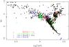 |
Fig. 1 HR diagram of the ELODIE library used as reference within the ETOILE code. |
Table B.1 lists the ELODIE reference stars used in the present work, and the stellar parameters adopted for them. They are represented in the HR diagram with colour codes depending on the metallicity in Fig. 1. Table B.2 lists the field validation stars observed with CARELEC, and Table B.3 the cluster stars observed with CFHT/MOS together with the atmospheric parameters adopted for them.
The ETOILE reference library includes Hipparcos stars having parallaxes with a relative error lower than 30%. Their absolute magnitudes MV were derived from the Tycho-2 VT apparent magnitude, transformed into V Johnson band, and these stars were used as reference stars for MV. Extensive tests to estimate the internal precision and external accuracy of MV determined that way, through the TGMET code, are presented in Soubiran et al. (2003, 2008). The validation of MV estimated through ETOILE is presented in Sect. 3.3. As can be seen in Fig. 1, representing the distribution of the reference library in the plane log (Teff) − MV, there are numerous stars covering the whole HR diagram and metallicity range (except metal-poor stars at the tip of the giant and asymptotic branches), to be used as reference stars for MV. This suggests that the reference library is representative of the program stars. It is less suited for the CFHT validation stars and in particular M 5 and M 92 stars, which comprise a large fraction of metal-poor stars from the tip of the giant and asymptotic branches.
A few program stars with inaccurate parameters, usually due to too low a signal to noise ratio, were discarded. Table A.2 gives the results of ETOILE for the 346 stars (162 FM3 and 184 FM5) kept for the scientific analysis: spectroscopic effective temperatures, surface gravities log g, metallicities [Fe/H], absolute magnitudes MV, radial velocities and photometric effective temperatures (used for validation only). Figure 2 gives a representation of the sample stars in the HR diagram.
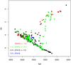 |
Fig. 2 HR diagram of the sample stars. |
3.3. Validation of stellar parameters
We have performed a series of tests in order to validate the results obtained with the code ETOILE.
3.3.1. Validation of results from CARELEC data
We tested 45 validation stars (Table B.2), running ETOILE on all the ELODIE reference library, and preventing the comparison with the star itself when it was both a reference and present in the validation set. We have then computed the mean values and 1-σ dispersion, as well as median and quantiles4 of the error distributions for Teff, log g, [Fe/H] and MV. The results obtained for the mean, 1σ dispersion, median and quantiles are given in Table 2. The atmospheric parameters of the validation stars come from various sources, extracted from the [Fe/H] catalogue (Cayrel de Strobel et al. 2001), and averaged. Their absolute magnitude have been estimated from their Hipparcos parallax only if the error was lower than 30%.
ETOILE performances for CARELEC validation stars.
Effective temperatures for validation stars with [Fe/H] > −2.0 exhibit no significant bias or trend; among the 6 validation stars with [Fe/H] < −2.0, 4 have temperatures overestimated by 200 to 400 K. These metal-poor stars are also mostly cool stars with bibliographic temperatures around 4500 K. Errors in gravity appear higher for giants than for dwarfs, and also higher for the lower metallicities. Importantly, there is no confusion of identification between giants and dwarfs.
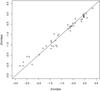 |
Fig. 3 Comparison of the metallicities determined with ETOILE with those compiled from the literature, for the validation stars observed with CARELEC. |
Figure 3 shows the metallicities estimated by ETOILE versus bibliographic, for the 45 validation spectra, as a function of bibliographic metallicities. There is a trend, with metallicities of metal-rich stars slightly underestimated (by about −0.1 dex at [Fe/H] = 0) and the metallicities of metal-poor stars overestimated (by about + 0.3 dex at [Fe/H] < −2.2). Among the 45 validation stars, 41 have their absolute magnitudes known from Hipparcos parallaxes. The overall 1-σ precision derived for these stars is 0.60 ± 0.07, corresponding to +32% and −24% error on the distances when the absolute magnitudes are respectively underestimated and overestimated. The 41 validation stars present a bias on MV of 0.2 mag, corresponding to a compression of the distances by −8.8%. Moreover, a few dwarfs have absolute magnitudes preferentially underestimated (and therefore their distances overestimated), while a few giants have it preferentially overestimated (and therefore, their distances underestimated).
The validation set was used to estimate the precision, bias and trends of ETOILE in analysing the CARELEC data. Yet, we considered that it was not suited (not large enough, not exactly the same proportion of dwarfs, sub-dwarfs, giants, metallicity distribution, etc.) to derive corrections for the bias and trends. Therefore, no corrections have been applied to the parameters of the program stars.
3.3.2. Validation of results from CFHT data
Using 72 spectra of 51 validation stars (Table B.3) from the open cluster M 67 (21 spectra) and the globulars M 71 (29 spectra), M 5 (17 spectra) and M 92 (5 spectra) we estimated the performance of ETOILE with CFHT spectra. For our validation stars, the bibliographic metallicities and absolute magnitudes are usually much more accurate than the effective temperatures and surface gravities. We therefore focused this part of the work on the performance of ETOILE in determining the metallicities and absolute magnitudes of CFHT spectra. The mean values and 1-σ dispersion, as well as median and quantiles of the error distributions for [Fe/H] and MV are given in Table 3.
ETOILE performances for CFHT validation stars.
Figure 4 shows the estimated metallicities as a function of bibliographic metallicities for 72 spectra of the 51 validation stars, listed in Table B.3. Each vertical line corresponds to one cluster, from right to left M 67 ([Fe/H]bib = 0.0 dex), M 71 ([Fe/H]bib = −0.73 dex), M 5 ([Fe/H]bib = −1.27 dex) and M 92 ([Fe/H]bib = −2.28 dex). The bibliographic metallicities of the globular clusters are given in Table A.3, whereas for M 67 we adopted the metallicity of [Fe/H] = 0.0 from An et al. (2009).
ETOILE recovered the mean metallicity of M 67 without statistically significant bias and with a 1-σ dispersion of 0.17 dex (similar to the performance for CARELEC).
The mean metallicity estimated for M 71 is about 0.2 dex above the bibliographic metallicity. The bulk (23 among 26) of M 71 spectra show a dispersion of 0.09 dex. The 3 spectra remaining show much larger errors. As the observation and selection of the validation stars were made several years ago, we revised their cluster membership probability with more recent material. Three spectra (2 of KC-223 and 1 of KC-124 not shown in Fig. 4), were found to be non-members (with 0% membership probability) based on the revised list by Cudworth (1985), Cudworth (2006, priv. comm.), and studies by Alves-Brito et al. (2008). The three “outlier” spectra in Fig. 4 correspond to 2 stars KC-370 (75% membership probability) and KC-200 (86% membership probability). We considered the membership probability of these stars high enough to keep them in the estimate of the performances.
The metallicities found for M 5 spectra exhibit no significant bias, but the 1-σ dispersion is very large: 0.36 dex (much larger than for the 3 other clusters). Here also, we reassessed the membership probability and eliminated 3 stars (I-52, III-44, IV-61, not shown in the Fig. 4), based on the identifications by Cudworth (1979). Another 3 having low (but non-null) membership probability may be non-members, but are included in Fig. 4 and in the performance estimate. For several stars no recent membership probability was available and we were therefore unable to reassess the status of these stars.
The metallicities for the M 92 spectra are overestimated by about 0.3 dex and show a “small” 1-σ dispersion of 0.06 dex.
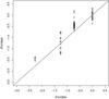 |
Fig. 4 Comparison of the metallicities determined with ETOILE with those compiled from the literature, for the validation stars observed with the CFHT/MOS. |
The absolute magnitude estimated by ETOILE for the validation stars exhibits a bias of about 1 mag leading to underestimating the distances by −37% and a 1-σ dispersion of 1.1 mag (corresponding to errors of −40% / +66% on the distances). The errors derived for the validation stars, may not be representative of the errors on the program stars. This can be explained as follows. In Fig. 1 we see that the stars of the ELODIE library contain only very few metal-poor stars of the red giant branch tip (RGB tip) or of the asymptotic branch tip, showing mostly giants at the clump level. On the contrary, the validation set contains a significant fraction of RGB/asymptotic branch tip stars (as those are bright and easier to observe in faint globular clusters, than other giants fainter down the giant branch). ETOILE is limited in the determination of the parameters to the parameter space of the reference library it uses. It therefore occurs that it identified the RGB/asymptotic branch tip validation stars as fainter giants, and as a consequence underestimates their absolute magnitude by up to 2 to 3 mag. Yet, the over-representation of giant and asymptotic branch stars in the validation stars is not representative of the program stars. The program stars should not suffer from the lack of analogs in the reference library as the validation stars do. Therefore, we expect that the statistical error on the estimation of the absolute magnitudes of the program stars is better than the one derived from the validation dataset. It is reassuring that the CARELEC validation spectra (covering a similar wavelength range) which are much more representative of the program spectra, present a significantly smaller bias of 0.2 mag, corresponding to −8.8% on the distances. In any case, in the interpretation of the characteristics of the program stars we first divide the dataset in 3 large bins of distances to minimise the number of stars that will be placed in the wrong bin of distance.
As for CARELEC spectra we decided to apply no correction to the parameters of the program stars.
3.4. Photometric versus spectroscopic temperatures
SDSS photometry was available for some of the program stars and was used to derive photometric effective temperatures (cf. Sect. 2.2). Figure 5 compares the photometric temperature with the spectroscopic temperature derived by ETOILE. For stars with photometric temperatures larger than 4750 K, the photometric and spectroscopic temperatures are in good agreement and compatible with the 1-σ dispersion of 165 K derived with the CARELEC validation stars. Below 4750 K, and in particular around 4250 K (photometric), the spectroscopic temperatures are systematically higher than the photometric ones. This is likely due to the hydrogen Hβ lines (4861 Å, present in both CARELEC and CFHT spectra) which is a very good temperature indicator above about 5000 K, and which quickly looses its sensitivity to temperature below this threshold. The CARELEC validation set includes 10 stars with bibliographic temperatures cooler than 4750 K. On average ETOILE overestimates the temperatures of this sub-group by 185 K. For the same sub-group, the metallicities determined by ETOILE show no significant bias and are determined with a 1-σ precision of 0.21 dex (slightly worse than the precision for the whole sample: 0.18 dex, see Sect. 3.3.1).
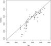 |
Fig. 5 Effective temperature Teff derived with the ETOILE code, compared with photometric temperatures based on SDSS colours. |
3.5. Distances and galactic velocities
Distances have been computed for all the target stars from V magnitudes and the ETOILE MV values. Due to the high galactic latitude of the two fields, the interstellar absorption has been neglected in the computation of the distances. Proper motions, distances and radial velocities have been combined to compute the 3 velocity components (U,V,W) with respect to the Sun (U positive toward the galactic centre). The galactic position (X,Y,Z) was also computed. Figure 6 shows the distribution of the sample in the X,Z plane.
For the CFHT sample, since radial velocities are not available, galactic velocities were derived only for the two components given by the proper motions, i.e. U and V for the field M 3 and Usin(47°) − Wcos(47°), hereafter UW, and V for the field M 5.
In Table A.3 are given the galactic distances X, Y, Z in parsecs, and the galactic velocities U, V, W when available or UW, V in km s-1.
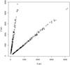 |
Fig. 6 X vs. Z (pc) of the sample stars. |
4. Results and discussion
4.1. Height versus metallicity
Figure 7 shows the height z above the Galactic plane of the sample stars as a function of their metallicity. The height z is expressed in parsecs. Both fields are represented: FM3 as red dots and FM5 as blue triangles. Figure 8 presents the combined distribution of metallicities for FM3 plus FM5 for 3 intervals of heights: z < 1 kpc, 1 < z < 2 kpc and 2 < z < 5 kpc. The histograms in Fig. 8 combine stars from two widely separated fields. In order to check whether it is legitimate to combine them, we ran a Kolmogorov-Smirnov (KS) test, for each height interval, comparing the metallicity distributions in FM3 and in FM5. The p-values of the KS tests are 0.67, 0.31 and 0.67. The KS tests therefore indicate that FM3 and FM5 present statistically similar metallicity distributions and can be combined for analysis.
In both figures, several groups of stars can be distinguished. These can be associated with the canonical Galactic populations: the thin disc here peaks around [Fe/H] ~ −0.1 dex, the thick disc displays a mode in metallicity around −0.45 dex (for z < 1 kpc), ~−0.55 dex (for 1 < z < 2 kpc) and ~−0.65 dex (for 2 < z < 5 kpc), the inner halo is visible above 3 kpc.
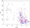 |
Fig. 7 Height z (from the Galactic plane) of the sample stars versus metallicity. Red circles correspond to the M 3 field stars, blue triangles to the M 5 field stars. |
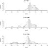 |
Fig. 8 Histogram of metallicities of the sample stars, including M 3 and M 5 field stars together for heights from the galactic plane 0 < z < 1 kpc, 1 < z < 2 kpc and 2 < z < 5 kpc. |
4.1.1. Thin-thick disc interface
In both Figs. 7 and 8 the ratio of thin disc stars (defined as the stars that cluster around [Fe/H] ~ −0.1 dex) to thick disc stars (clustering around [Fe/H] ~ −0.5/ −0.6 dex) decreases significantly between the “lower” bin z < 1 kpc and the “intermediate” bin 1 < z < 2 kpc. The formalism “classically” used to model the spatial vertical profile of the disc, i.e. the sum of two populations (thin plus thick disc) with different vertical scale heights (such that the ratio of the two populations vary monotonically with height), also holds here for the Metallicity Distribution Function (MDF) of the disc as a function of height. It should be noted that recent studies based on SDSS data (Ivezić et al. 2008; Bond et al. 2010) reach a somewhat different conclusion. This question is discussed in Sect. 4.3.
A few stars with “typical” thin-disc metallicities, i.e. −0.3 < [Fe/H] < 0 are still present in the 2 < z < 5 kpc height bin. Lee & Beers (2009), Carollo et al. (2010) and Bond et al. (2010) have also reported the presence of thin-disc type stars at several kpc above the Galactic plane.
4.1.2. Thick disc vertical metallicity gradient
The thick disc is the dominant population in the height bins 1 < z < 2 kpc and 2 < z < 5 kpc. In Fig. 8, the mode of the thick disc is located in the metallicity bin −0.5 < [Fe/H] ≤ −0.4 dex for heights below 1 kpc, in the bin ] −0.6, −0.5] dex for the height bin 1 < z < 2 kpc and in the bin ] −0.7, −0.6] dex for the bin 2 < z < 5 kpc. We checked that the shift with height of the mode of the thick disc MDF toward lower metallicities was not an artifact resulting from the combination of 2 datasets observed with two different spectrographs. We examined the MDFs of the CARELEC and CFHT sub-samples separately. The shift is visible in both sub-samples, with a poorer contrast due to the smaller statistics.
The observed decrease in metallicity with increasing height of the mode of the thick disc MDF raises several questions. What is the statistical significance of this decrease? If significant, does it trace a gradient in the thick disc or does it result from the variation with height of the contamination by the “metal-poor” tail of the thin disc MDF? FM3 stars are distributed almost perpendicular to the Galactic plane (FM3 latitude is b = 80°), but FM5 stars have a similar radial distance from the Sun toward the Galactic centre as distance above the Galactic plane (FM5 latitude is b = 46°). Therefore, if the metallicity shift is both significant and not induced by the thin disc, is it a vertical effect, a radial effect or a combination of both?
In order to obtain more precise estimates of the thick disc modes, the MDFs in the 3 height bins were convolved with a Gaussian kernel. The convolution transforms the discrete distributions into continuous distributions and allows the derivation of the modes independently of any binning assumptions (on the contrary to the histograms). The convolution also smooths out the noise-induced small scale structures due to the moderate statistics of our sample. The convolution kernel, σ = 0.08 dex, was chosen empirically as large enough to smooth the small scale noise peaks, but small enough to avoid increasing significantly the contamination of the thick disc by the thin disc and vice-versa. The 1-sigma error bars on the locations of the modes were estimated by bootstrap, generating, for each height bin, 5000 datasets; each dataset made of N stars randomly selected among the N stars in each height bin (N equals 175, 94 and 68 respectively in the 3 height bins). The values estimated for the modes are: −0.48 ± 0.02 dex (0 < z < 1 kpc), −0.55 ± 0.03 dex (1 < z < 2 kpc) and −0.62 ± 0.03 dex (2 < z < 5 kpc). Before evaluation of the impact of the thin disc contamination, the significance of the difference of metallicity between the bottom and top bins is 3.7σ, where σ, calculated as the quadratic sum of the individual errors, equals 0.037 dex.
To evaluate the impact of the thin disc on the location of the mode of the thick disc, the thin disc MDFs were modelled for each height bin and subtracted from the observations. The shape of the MDF of the thin disc in the 2 directions (l = 51°, b = 80° and l = 5°, b = 46°) was simulated with the Besançon Galaxy model (Robin et al. 2003) using the selection criteria: 12.5 < V < 18 and the appropriate cut in height above the Galactic plane. The synthetic thin disc MDFs were then: (i) shifted by −0.05 dex5 in order that the locations of the modes of the thin disc coincide in the synthetic sample and in our program stars; (ii) convolved with the same Gaussian kernel as the program stars; (iii) normalised to the number of stars measured in the mode of the thin disc of the program stars; and (iv) subtracted from the smoothed MDFs of the program stars. The subtraction of the contribution of the thin disc shifts the mode of the thick disc from −0.48 to −0.51 dex (0 < z < 1 kpc), from −0.55 to −0.56 dex (1 < z < 2 kpc) and has a negligible impact on the mode above 2 kpc. The median height of the stars in the bottom bin is 580 pc and 2630 pc for the top bin. We therefore observe a decrease of the value of the mode of the thick disc MDF of −0.11 ± 0.037 dex (corresponding to a 3.02σ statistical significance) over 2050 pc.
We observe a shift toward lower metallicities of the mode of the thick disc with increasing height. But what is the nature of this shift? Is it a constant gradient or is it a more complex behaviour? To address this question, the combined FM3 and FM5 sample was divided into 6 height bins, each of 500 pc. In each bin, (i) the sub-sample was convolved by a Gaussian kernel, as described above; (ii) the contribution of the thin disc was modelled with the Besançon Galaxy model (Robin et al. 2003) and subtracted6 from the continuous Metallicity Distribution Function; and (iii) the value of the mode of the MDF was measured. The results are given in Table 4 and displayed in Fig. 9. A gradient was fitted to the results by weighted least square and is shown as a red line on Fig. 9. The data are well matched by a metallicity gradient, ∂ [Fe/H] /∂z = −0.068 ± 0.009 dex kpc-1 with an intercept [Fe/H] (z = 0) = −0.460 ± 0.014 dex.
As presented in Sect. 3.3.1, the distances derived for the 41 CARELEC validation stars were, on average, underestimated by 8.8%. Increasing the distances of the program stars by 9.6% would reduce the metallicity gradient to ∂ [Fe/H] /∂z = −0.060 ± 0.008 dex kpc-1.
Thick disc metallicity mode as a function of height.
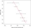 |
Fig. 9 Mode of the thick disc Metallicity Distribution Function as a function of height above the Galactic plane. The red line represents the weighted best fit gradient. |
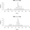 |
Fig. 10 Histogram of metallicities of the sample stars for the M 3 field (upper panel) and M 5 field (bottom panel), for heights from the galactic plane 2 < z < 4 kpc. |
To establish whether the observed gradient has a radial origin or a vertical one or a mix of both, we separated FM3 and FM5. Figure 10 presents the MDF of FM3 stars (top) and FM5 stars (bottom) in the height range 2 < z < 4 kpc. The mean location of the FM3 sub-sample is x = 0.3 kpc (x measured from the Sun toward the Galactic centre) and z = 2.7 kpc, and the one of FM5 is x = 2.5 kpc and z = 2.6 kpc. In both top and bottom histograms, the thick disc mode is at [Fe/H] = −0.65 dex and the distributions around the modes are very similar. This is confirmed by the comparison of the 2 distributions using a Kolmogorov-Smirnov test which yielded a p-value of 0.27. The 2 distributions were then convolved with the Gaussian kernel, as described above, and the locations of the modes were evaluated: −0.60 ± 0.08 dex (FM3) and −0.63 ± 0.05 dex (FM5). The two modes are very close (much closer than the difference of the modes between the bottom and top bins), but the error bars are too large to exclude unambiguously the possibility of a radial origin.
To investigate further the radial or vertical origin of the gradient, we compared the statistical significance of the 2 “extreme” hypotheses, a purely vertical versus a purely radial effect. The statistical significance of the purely vertical origin is provided by the comparison of the bottom and top height bins for the samples combining FM3 and FM5. It has been evaluated above to be 3.02σ. To establish the statistical significance of the purely radial origin, the FM3 stars in the height range 0 < z < 4 kpc were compared to the FM5 stars in the height range 2 < z < 4 kpc. After correction for the thin disc contamination, the 2 thick disc modes were measured at −0.58 ± 0.04 (FM3, 0 < z < 4 kpc) and −0.63 ± 0.05 (FM5, 0 < z < 2 kpc). The statistical significance of a radial origin is 0.73σ, where σ = 0.066 dex. The vertical origin is therefore statistically strongly favoured.
Figures 7 and 8 present a gap in metallicity, between [Fe/H] = −1.2 and −1.0, below 2.5 kpc. This could trace a decline of the number of thick disc stars at its low metallicity end (coupled with the modest statistics of our sample). Another aspect that could also play a role here is that there is a very localised absence of dwarfs stars around Teff = 5500 K and metallicity −1 < [Fe/H] < −1.5 in the reference library used by ETOILE (there are cooler and warmer dwarfs). As a consequence ETOILE may either under- or overestimate a bit the metallicity of stars falling in the local hole of the library.
4.1.3. Metal-poor stars
In Fig. 7, one can see seven stars grouped within a “small” interval of metallicity, −1.4 < [Fe/H] < −1.2 and distributed in height from 0.9 to 2.5 kpc above the Galactic plane. The location of these stars in the height-metallicity diagram make them compatible with a metal-poor tail of the thick disc or with the inner halo or with the metal weak thick disk – MWTD (Ivezić et al. 2008; Carollo et al. 2010). The very small statistics do not allow us to determine the parent population(s) of these stars.
Inner halo stars are visible above 2.5 kpc in the metallicity range −2.1 < [Fe/H] < −1.4.
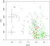 |
Fig. 11 Height as a function of metallicity, as in Figure 7, but here the colour code refers to velocities. Symbols: green circles: V > −50; red triangles: −100 < V < −50; blue crosses: −150 < V < −100; black tilted crosses: V < −150 km s-1. |
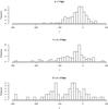 |
Fig. 12 V distribution functions in the same 3 intervals of height as in Figs. 8: 0 < z < 1 kpc, 1 < z < 2 kpc and 2 < z < 5 kpc. |
4.2. Rotational velocity versus metallicity
Figure 11 presents the height of the stars as a function of metallicity, with symbols and colours encoding the velocity V: green circles: V > −50; red triangles: −100 < V < −50; blue crosses: −150 < V < −100; black tilted crosses: V < −150 km s-1. Figure 12 shows the V velocity distribution function in the three height intervals: 0 < z < 1 kpc, 1 < z < 2 kpc and 2 < z < 5 kpc. Figure 13 presents the circular component of the velocity, V, of sample stars as a function of their metallicity. Both FM3 (as red circles) and FM5 (as blue triangles) stars are shown. The stars are divided in three intervals of height z: z < 1 kpc, 1 < z < 2 kpc, 2 < z < 5 kpc. The three top plots share the same scale and boundaries. As a consequence, some non or counter-rotating stars fall outside a plot. “Full-view” versions of the plots are presented at the bottom of the figure.
As in Fig. 7, the canonical populations can be identified in these figures. The thin and thick discs are both visible, respectively around [Fe/H] = −0.1 and [Fe/H] = −0.45/ −0.55/ −0.65 dex. Here also, the ratio of thin disc to thick disc stars significantly decreases from the lower bin (z < 1 kpc) to the intermediate bin (1 < z < 2 kpc).
Among the seven stars discussed in Sect. 4.1 as possibly belonging to the thick disc, inner halo or metal weak thick disk, one is significantly counter rotating and very likely belongs to the halo. The rotational velocities of the 6 remaining stars and the very small statistics, prevent removing the degeneracy and determining their parent population(s).
In the high height bin (2 < z < 5 kpc) inner halo stars are visible at metallicities [Fe/H] < −1.5 dex. The mean rotation of the inner halo stars is −114 km s-1, corresponding to Vφ = 106 km s-1. From Fig. 9 of Carollo et al. (2010), a Vφ of a few tens of km s-1 is expected at a few kpc above the plane. The excess of rotation of our inner halo sub-sample is likely due to the small statistics.
4.3. Thick disc metallicity, gradient and interfaces in recent studies
Soubiran et al. (2003) collected high resolving power (R = 42 000) low signal to noise (S/N ~ 20) spectra for 400 Tycho-2 stars (Høg et al. 2000a,b) distributed from 200 to 800 parsecs above the Galactic plane in the direction of the North Galactic Pole. They deconvolved the thin and thick disc populations at different heights and measured a mean metallicity for the thick disc of ⟨ [Fe/H] ⟩ = −0.48 ± 0.05 dex in the height bin [400,800] pc.
Allende Prieto et al. (2006) analysed the low resolving power (R ~ 2000) spectra of 22 770 F and G-type stars from the SDSS 3rd data release (Abazajian et al. 2005). The bulk of the sample probes the height range [1,10] kpc under and above the Galactic plane and the full sample extends up to ~100 kpc. In the height interval [1,3] kpc the thick disc peaks at about −0.7 dex (with a binning of 0.2 dex). Excluding the stars with [Fe/H] < −1.2 dex they derived a thick disc mean metallicity of ⟨ [Fe/H] ⟩ = −0.685 ± 0.004 dex for the G-type stars in the height bin 1 < | z | < 3 kpc.
Siegel et al. (2009) analysed UBVRI photometry of 368 stars contained in the Selected Area 141 near the south Galactic pole and probing the disc and halo to about 15 kpc below the Galactic plane. They compared several Galaxy models to their data and found as a best fit the model with a thick disc mean metallicity of −0.78 dex.
Soubiran et al. (2003) thick disc metallicity in the height range 0.4 < z < 0.8 kpc, ⟨ [Fe/H] ⟩ = −0.48 ± 0.05 dex is in good agreement with ours for the height range 0.5 < z < 1.0 kpc, [Fe/H] = −0.52 ± 0.04 dex. The mean metallicity derived by Allende Prieto et al. (2006) for the height interval 1 < | z | < 3 kpc, ⟨ [Fe/H] ⟩ = −0.685 ± 0.004 dex, is on the metal-poor edge of the range of metallicity that we obtain. It is close to the metallicity that we estimate for the height range 2.5 < z < 3 kpc, −0.67 ± 0.09 dex and more deficient by about 0.1 dex, than the mode of our sample for the interval 1 < z < 3 kpc, −0.59 ± 0.02 dex. We can note that in this height interval, stars between 1 and 2 kpc represent about 2/3 of our sample, while from Allende Prieto et al. (2006)’s Figs. 11 and 12, their star counts seem similar between [1,2] kpc and [2,3] kpc. The mean metallicity derived by Siegel et al. (2009), −0.78 dex, is about 0.2 dex more metal-poor than the metallicity that we obtain in the height interval 1 < z < 3 kpc. It should be noted that the 3 studies discussed here estimate the mean value of the thick disc MDF, while we evaluate the value of the mode. If the thick disc MDF was to be asymmetric, then the mean and mode would not coincide. Moreover, these 3 studies, as well as ours, rely on different observables and different methods to derive the metallicity of the stars. As a consequence, there might be differences between the four metallicity scales.
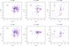 |
Fig. 13 Circular component of velocity V(km s-1) vs. metallicity [Fe/H], given in 3 height intervals: 0 < z < 1 kpc, 1 < z < 2 kpc and 2 < z < 5 kpc. Symbols: red circles: M 3 field; blue triangles: M 5 field. The top plots share the same scales and boundaries. “Full-view” versions of the plots are displayed at the bottom. |
Allende Prieto et al. (2006) observe no metallicity gradient in the thick disc in the height range 1 < | z | < 3 kpc and estimate an upper limit for the gradient of 0.03 dex kpc-1.
Siegel et al. (2009) compared their observations to models without and with a thick disc vertical metallicity gradient. Their favoured model presents no gradient. Yet, one of the models with a gradient of −0.05 dex kpc-1 is also compatible with their observations, in particular in the height interval where the thick disc is the dominant population, 1 < z < 4 kpc.
Allende Prieto et al. (2006), Siegel et al. (2009) and our study all three present similar precisions in the estimation of individual metallicities of the order of 0.20 dex and show also some systematics. The next step, to confirm or not the presence of a vertical metallicity gradient in the thick disc, is to improve the precision as well as the accuracy on the individual measures by acquiring high resolving power spectra, e.g. R ≥ 20 000 for a sample probing the height interval 1 < z < 3 kpc.
Ivezić et al. (2008) analysed 110 363 stars selected in the SDSS Stripe 82 to study the chemical and kinematical properties of the disc plus halo system from a few hundred parsecs to 7 to 9 kpc above the Galactic plane (the height reached is a function of the direction on the celestial sphere). In particular, they established the MDF of the disc plus halo system as a function of height. This MDF has been slightly revised in the next paper of the series, Bond et al. (2010) (see their Appendix A), using an improved determination of the metallicities of the metal-rich stars up to [Fe/H] = −0.2 dex. Figure A.4 of Bond et al. (2010) presents 4 MDFs for 4 bins of height: 0.8 < z < 1.2 kpc, 1.5 < z < 2 kpc, 3 < z < 4 kpc and 5 < z < 7 kpc. It is interesting to compare their Fig. A.4 with Fig. 8 in the present article.
At heights in the range 1 < z < 2 kpc, their MDFs peak around −0.8 dex, close to the mean value derived by Siegel et al. (2009) and about 0.2 dex more metal poor than our estimation of the metallicity of the mode.
On the “metal-rich” side, our MDF shows a significant extended tail (that we interpret as the thin disc peaking around [Fe/H] ~ −0.1 dex). This extended tail/secondary peak is not present in Bond at al.’s MDF in which (i) the fraction of stars with [Fe/H] > −0.3 dex is very small and (ii) the metal-rich wing of the disc MDF shows no secondary peak. As noted by Bond et al. (2010) in their Appendix A.1, their metallicity calibration range extends to [Fe/H] ~ −0.2. The authors suggest that their metallicities could be underestimated by 0.2−0.3 dex at [Fe/H] = 0. This metallicity calibration effect may be (one of) the reason(s) for the difference observed on the metal-rich side.
This difference in the shape of the MDF on the metal-rich side, certainly explains the other difference already noted in Sect. 4.1. Ivezić et al. (2008) and Bond et al. (2010) found that “the disk metallicity distribution varies with z such that its shape remained fixed, while its median μD varies (...)”. As discussed in Sect. 4.1 we find a variation of the shape of the disc MDF as a function of height, due to the decrease of the strength of the peak at [Fe/H] = −0.1 dex (that we interpret as thin disc stars) with respect to the thick disc peak.
4.4. Discussion: thick disc gradient versus formation scenarios
As presented in the introduction, there are currently several mechanisms and scenarios that can explain the formation of the thick disc. Some of them predict a vertical metallicity gradient while others do not.
In the scenario in which the thick disc is formed from stars accreted during a merger, the final vertical dispersion of the accreted stars is independent of their metallicity. Therefore, no metallicity gradient is expected.
Brook et al. (2005) used the cold dark matter chemo-dynamical galaxy formation code GCD + (Kawata & Gibson 2003) to simulate the formation of four Milky-Way-like galaxies. In the four cases, a thick disc appears by accretion of gas-rich building blocks and in-situ (i.e. in the galactic disc) formation of stars. From their Fig. 8, one can see that very little vertical metallicity gradient is present in any of the four thick discs.
Quinn et al. (1993) performed N-body simulations to study the accretion of “small” (i.e. 4 to 20% of the disc mass) satellite(s) by a large spiral galaxy. The satellite(s) “heat” the initial thin disc by dynamical friction and produce a thick disc. Some stars, stripped from the satellite, also contribute to the thick disc, while the core of the satellite sinks in the nucleus of the disc. The original thin disc does not survive the merger phase, but is re-built later by secondary processes. If the initial thin disc was presenting a vertical metallicity gradient, this gradient is preserved and can even be enhanced by the merging event(s), because “the least tightly bound disc particles suffer some of the largest increases in scale height”.
In the secular formation scenario of the thick disc proposed by Schönrich & Binney (2009a,b), the stars are “continuously” heated and radially mixed by spiral arms and molecular clouds. Older and more metal-poor stars are more subject to vertical heating than younger stars. One can therefore expect a vertical metallicity gradient in this case. We note that these points are not explicitly addressed in the two papers.
5. Summary and conclusion
In this article we investigate the properties of the thick disc as a function of the height above the Galactic plane and we examine the interfaces between the thin disc, thick disc and halo. To conduct this study, 421 spectra of field stars, spanning the magnitude range 12.5 < V < 18, were selected, with no kinematical or chemical bias, in the proper motion catalogues of Soubiran (1992) (in the direction l ~ 51°, b ~ 80°) and Ojha et al. (1994) (in the direction l ~ 5°, b ~ 46°). These stars were observed with the low resolution spectrographs CARELEC (Δλ = 3.5 Å) and MOS-SIS (Δλ = 6.25 Å), respectively installed at the Haute-Provence observatory and on the Canada-France-Hawaii telescope. The radial velocities (for CARELEC spectra only), effective temperatures, surface gravities, metallicities and absolute magnitudes were extracted from the spectra using the ETOILE software. The distances were deduced from the “spectroscopic” absolute magnitudes, allowing us to transform the proper motions into linear velocities.
The MDF of the (thin-thick-)disc-halo system was derived for several intervals of height above the Galactic plane.
The ratio of stars with thin-disc metallicities over stars with thick disc metallicities strongly decreases with height between the first and the second kilo-parsec above the Galactic plane. This is consistent with the approach classically used to model the disc density as a function of height: i.e. a superposition of 2 discrete populations with 2 different scale heights.
The examination of the disc MDF at several heights above the Galactic plane, shows a vertical metallicity gradient in the thick disc ∂ [Fe/H] /∂z = −0.068 ± 0.009 dex.kpc-1. The presence or absence of a thick disc vertical metallicity gradient is discussed for some formation scenarios. The accretion of gas-rich building blocks (Quinn et al. 1993) or the secular evolution of the disc as stars are dynamically heated as well as radially mixed by spiral arms and molecular clouds (Schönrich & Binney 2009a,b) are compatible with a thick disc vertical metallicity gradient.
The next step is now to confirm and, if confirmed, to characterise more precisely the thick disc vertical metallicity gradient, using high resolution spectra. Moreover, studies in the solar neighbourhood have shown that thick disc stars are α-element-enhanced with respect to thin disc stars (Fuhrmann 1998, 2004, 2008; Prochaska et al. 2000; Mishenina et al. 2004; Soubiran & Girard 2005; Reddy et al. 2006; Feltzing et al. 2003; Bensby et al. 2003, 2004, 2005, 2007; Meléndez et al. 2008; Alves-Brito et al. 2010). To set additional constraints on the formation of the thick disc, it is of great interest to now look at how this α-element enhancement evolved with distance outside of the solar neighbourhood and in particular with height above the Galactic plane.
In these scenarios, the dynamical heating is the dominant process, but the accreted material usually ends up, at least partly, as a (minor) contribution to the thick disc, e.g. in Read et al. (2008) accreted stars contribute to 10 to 50% of the thick disc.
Updated in 2003 as given in http://www.physics.mcmaster.ca/Globular.html.
The radial velocities of the validation stars were derived with both a single template and templates corresponding to their known atmospheric parameters. No significant improvement was obtained with the second approach.
We used as a robust estimator of the standard deviation: the half difference between the 84.15th percentile of the sorted distribution of errors and the 15.85th percentile of the same distribution. This estimator gives low weight to the outliers.
Only in the first height bin.
The thin disc, modelled with the Besançon Galaxy model, significantly affects the mode of the thick disc up to 1.5 kpc and was only subtracted in the 3 first height bins.
Acknowledgments
The authors would like to thank Misha Haywood, Frédéric Arenou and Ana Gómez for very stimulating and helpful discussions and advice. B.B. acknowledges partial financial support by CNPq and Fapesp. We are grateful to the referee for his/her very fruitful comments and suggestions.
References
- Abadi, M. G., Navarro, J. F., Steinmetz, M., & Eke, V. R. 2003, ApJ, 597, 21 [NASA ADS] [CrossRef] [MathSciNet] [Google Scholar]
- Abazajian, K., Adelman-McCarthy, J. K., Agüeros, M. A., et al. 2003, AJ, 126, 2081 [Google Scholar]
- Abazajian, K., Adelman-McCarthy, J. K., Agüeros, M. A., et al. 2005, AJ, 129, 1755 [Google Scholar]
- Abazajian, K. N., Adelman-McCarthy, J. K., Agüeros, M. A., et al. 2009, ApJS, 182, 543 [NASA ADS] [CrossRef] [Google Scholar]
- Allen de Prieto, C., Beers, T. C., Wilhelm, R., et al. 2006, ApJ, 636, 804 [NASA ADS] [CrossRef] [Google Scholar]
- Alonso, A., Arribas, S., & Martínez-Roger, C. 1999, A&AS, 140, 261 [NASA ADS] [CrossRef] [EDP Sciences] [Google Scholar]
- Alves-Brito, A., Schiavon, R. P., Castilho, B., & Barbuy, B. 2008, A&A, 486, 941 [NASA ADS] [CrossRef] [EDP Sciences] [Google Scholar]
- Alves-Brito, A., Meléndez, J., Asplund, M., Ramírez, I., & Yong, D. 2010, A&A, 513, A35 [NASA ADS] [CrossRef] [EDP Sciences] [Google Scholar]
- An, D., Pinsonneault, M. H., Masseron, T., et al. 2009, ApJ, 700, 523 [NASA ADS] [CrossRef] [Google Scholar]
- Arp, H. C., & Hartwick, F. D. A. 1971, ApJ, 167, 499 [NASA ADS] [CrossRef] [Google Scholar]
- Bensby, T., Feltzing, S., & Lundström, I. 2003, A&A, 410, 527 [NASA ADS] [CrossRef] [EDP Sciences] [Google Scholar]
- Bensby, T., Feltzing, S., & Lundström, I. 2004, A&A, 415, 155 [NASA ADS] [CrossRef] [EDP Sciences] [Google Scholar]
- Bensby, T., Feltzing, S., Lundström, I., & Ilyin, I. 2005, A&A, 433, 185 [NASA ADS] [CrossRef] [EDP Sciences] [Google Scholar]
- Bensby, T., Zenn, A. R., Oey, M. S., & Feltzing, S. 2007, ApJ, 663, L13 [CrossRef] [Google Scholar]
- Bond, N. A., Ivezić, Ž., Sesar, B., et al. 2010, ApJ, 716, 1 [NASA ADS] [CrossRef] [Google Scholar]
- Brook, C. B., Gibson, B. K., Martel, H., & Kawata, D. 2005, ApJ, 630, 298 [NASA ADS] [CrossRef] [Google Scholar]
- Buonanno, R., Corsi, C. E., & Fusi Pecci, F. 1981, MNRAS, 196, 435 [NASA ADS] [Google Scholar]
- Buonanno, R., Buscema, G., Corsi, C. E., et al. 1983, A&AS, 53, 1 [NASA ADS] [Google Scholar]
- Burkert, A., Truran, J. W., & Hensler, G. 1992, ApJ, 391, 651 [NASA ADS] [CrossRef] [Google Scholar]
- Carollo, D., Beers, T. C., Chiba, M., et al. 2010, ApJ, 712, 692 [NASA ADS] [CrossRef] [Google Scholar]
- Cayrel, R., Perrin, M., Barbuy, B., & Buser, R. 1991, A&A, 247, 108 [NASA ADS] [Google Scholar]
- Cayrel de Strobel, G., Soubiran, C., & Ralite, N. 2001, A&A, 373, 159 [NASA ADS] [CrossRef] [EDP Sciences] [Google Scholar]
- Cohen, J. G., Behr, B. B., & Briley, M. M. 2001, AJ, 122, 1420 [NASA ADS] [CrossRef] [Google Scholar]
- Cudworth, K. M. 1979, AJ, 84, 1866 [NASA ADS] [CrossRef] [Google Scholar]
- Cudworth, K. M. 1985, AJ, 90, 65 [NASA ADS] [CrossRef] [Google Scholar]
- Famaey, B., Jorissen, A., Luri, X., et al. 2005, A&A, 430, 165 [NASA ADS] [CrossRef] [EDP Sciences] [Google Scholar]
- Feltzing, S., Bensby, T., & Lundström, I. 2003, A&A, 397, L1 [NASA ADS] [CrossRef] [EDP Sciences] [Google Scholar]
- Fuhrmann, K. 1998, A&A, 338, 161 [NASA ADS] [Google Scholar]
- Fuhrmann, K. 2004, Astronom. Nachr., 325, 3 [NASA ADS] [CrossRef] [Google Scholar]
- Fuhrmann, K. 2008, MNRAS, 384, 173 [NASA ADS] [CrossRef] [Google Scholar]
- Gilmore, G., & Reid, N. 1983, MNRAS, 202, 1025 [NASA ADS] [CrossRef] [Google Scholar]
- Harris, W. E. 1996, AJ, 112, 1487 [NASA ADS] [CrossRef] [Google Scholar]
- Høg, E., Fabricius, C., Makarov, V. V., et al. 2000a, A&A, 357, 367 [NASA ADS] [Google Scholar]
- Høg, E., Fabricius, C., Makarov, V. V., et al. 2000b, A&A, 355, L27 [NASA ADS] [Google Scholar]
- Ivezić, Ž., Sesar, B., Jurić, M., et al. 2008, ApJ, 684, 287 [NASA ADS] [CrossRef] [Google Scholar]
- Johnson, H. L., & Sandage, A. R. 1955, ApJ, 121, 616 [NASA ADS] [CrossRef] [Google Scholar]
- Jones, B. J. T., & Wyse, R. F. G. 1983, A&A, 120, 165 [NASA ADS] [Google Scholar]
- Katz, D. 2001, J. Astron. Data, 7, 8 [Google Scholar]
- Katz, D., Soubiran, C., Cayrel, R., Adda, M., & Cautain, R. 1998, A&A, 338, 151 [NASA ADS] [Google Scholar]
- Kawata, D., & Gibson, B. K. 2003, MNRAS, 340, 908 [Google Scholar]
- Kazantzidis, S., Bullock, J. S., Zentner, A. R., Kravtsov, A. V., & Moustakas, L. A. 2008, ApJ, 688, 254 [NASA ADS] [CrossRef] [Google Scholar]
- Lee, Y. S., & Beers, T. C. 2009, BAAS, 41, 227 [NASA ADS] [Google Scholar]
- Ludwig, H., Bonifacio, P., Caffau, E., et al. 2008, Phys. Scr. T, 133, 014037 [Google Scholar]
- Meléndez, J., Asplund, M., Alves-Brito, A., et al. 2008, A&A, 484, L21 [NASA ADS] [CrossRef] [EDP Sciences] [MathSciNet] [Google Scholar]
- Mishenina, T. V., Soubiran, C., Kovtyukh, V. V., & Korotin, S. A. 2004, A&A, 418, 551 [NASA ADS] [CrossRef] [EDP Sciences] [Google Scholar]
- Montgomery, K. A., Marschall, L. A., & Janes, K. A. 1993, AJ, 106, 181 [NASA ADS] [CrossRef] [Google Scholar]
- Ojha, D. K., Bienayme, O., Robin, A. C., & Mohan, V. 1994, A&A, 290, 771 [NASA ADS] [Google Scholar]
- Perrin, M., Friel, E. D., Bienayme, O., et al. 1995, A&A, 298, 107 [NASA ADS] [Google Scholar]
- Prochaska, J. X., Naumov, S. O., Carney, B. W., McWilliam, A., & Wolfe, A. M. 2000, AJ, 120, 2513 [NASA ADS] [CrossRef] [Google Scholar]
- Prugniel, P., & Soubiran, C. 2001, A&A, 369, 1048 [NASA ADS] [CrossRef] [EDP Sciences] [Google Scholar]
- Prugniel, P., & Soubiran, C. 2004, unpublished [arXiv:astro-ph/0409214] [Google Scholar]
- Quinn, P. J., Hernquist, L., & Fullagar, D. P. 1993, ApJ, 403, 74 [NASA ADS] [CrossRef] [Google Scholar]
- Ramírez, S. V., & Cohen, J. G. 2003, AJ, 125, 224 [NASA ADS] [CrossRef] [Google Scholar]
- Read, J. I., Lake, G., Agertz, O., & Debattista, V. P. 2008, MNRAS, 389, 1041 [NASA ADS] [CrossRef] [Google Scholar]
- Reddy, B. E., Lambert, D. L., & Allen de Prieto, C. 2006, MNRAS, 367, 1329 [NASA ADS] [CrossRef] [Google Scholar]
- Reylé, C., & Robin, A. C. 2001, A&A, 373, 886 [NASA ADS] [CrossRef] [EDP Sciences] [Google Scholar]
- Robin, A. C., Reylé, C., Derrière, S., & Picaud, S. 2003, A&A, 409, 523 [NASA ADS] [CrossRef] [EDP Sciences] [Google Scholar]
- Sandage, A., & Walker, M. F. 1966, ApJ, 143, 313 [NASA ADS] [CrossRef] [Google Scholar]
- Schönrich, R., & Binney, J. 2009a, MNRAS, 396, 203 [NASA ADS] [CrossRef] [Google Scholar]
- Schönrich, R., & Binney, J. 2009b, MNRAS, 399, 1145 [NASA ADS] [CrossRef] [Google Scholar]
- Sekiguchi, M., & Fukugita, M. 2000, AJ, 120, 1072 [NASA ADS] [CrossRef] [Google Scholar]
- Siegel, M. H., Majewski, S. R., Reid, I. N., & Thompson, I. B. 2002, ApJ, 578, 151 [NASA ADS] [CrossRef] [Google Scholar]
- Siegel, M. H., Karataş, Y., & Reid, I. N. 2009, MNRAS, 395, 1569 [NASA ADS] [CrossRef] [Google Scholar]
- Skrutskie, M. F., Cutri, R. M., Stiening, R., et al. 2006, AJ, 131, 1163 [NASA ADS] [CrossRef] [Google Scholar]
- Sneden, C., Pilachowski, C. A., & Kraft, R. P. 2000, AJ, 120, 1351 [NASA ADS] [CrossRef] [Google Scholar]
- Soubiran, C. 1992, A&A, 259, 394 [NASA ADS] [Google Scholar]
- Soubiran, C., & Girard, P. 2005, A&A, 438, 139 [NASA ADS] [CrossRef] [EDP Sciences] [Google Scholar]
- Soubiran, C., Katz, D., & Cayrel, R. 1998, A&AS, 133, 221 [NASA ADS] [CrossRef] [EDP Sciences] [Google Scholar]
- Soubiran, C., Bienaymé, O., & Siebert, A. 2003, A&A, 398, 141 [NASA ADS] [CrossRef] [EDP Sciences] [Google Scholar]
- Soubiran, C., Bienaymé, O., Mishenina, T. V., & Kovtyukh, V. V. 2008, A&A, 480, 91 [NASA ADS] [CrossRef] [EDP Sciences] [Google Scholar]
- Soubiran, C., Le Campion, J., Cayrel de Strobel, G., & Caillo, A. 2010, A&A, 515, A111 [NASA ADS] [CrossRef] [EDP Sciences] [Google Scholar]
- Steinmetz, M., Zwitter, T., Siebert, A., et al. 2006, AJ, 132, 1645 [NASA ADS] [CrossRef] [Google Scholar]
- VandenBerg, D. A., & Clem, J. L. 2003, AJ, 126, 778 [NASA ADS] [CrossRef] [Google Scholar]
- Veltz, L., Bienaymé, O., Freeman, K. C., et al. 2008, A&A, 480, 753 [NASA ADS] [CrossRef] [EDP Sciences] [Google Scholar]
- Villalobos, Á., & Helmi, A. 2008, MNRAS, 391, 1806 [NASA ADS] [CrossRef] [Google Scholar]
- Villalobos, Á., Kazantzidis, S., & Helmi, A. 2010, ApJ, 718, 314 [NASA ADS] [CrossRef] [Google Scholar]
- Yanny, B., Rockosi, C., Newberg, H. J., et al. 2009, AJ, 137, 4377 [NASA ADS] [CrossRef] [Google Scholar]
- Zwitter, T., Siebert, A., Munari, U., et al. 2008, AJ, 136, 421 [NASA ADS] [CrossRef] [Google Scholar]
Appendix A: Program stars
Appendix A presents the parameters of the program stars.
CARELEC and CFHT program stars.
CARELEC and CFHT program stars: stellar parameters.
CARELEC and CFHT program stars: metallicities, positions and velocities.
Appendix B: Reference and validation stars
Appendix B presents the parameters of the reference and validation stars.
ELODIE library reference stars.
CARELEC validation stars.
CFHT validation stars.
All Tables
All Figures
|
Fig. 1 HR diagram of the ELODIE library used as reference within the ETOILE code. |
| In the text | |
|
Fig. 2 HR diagram of the sample stars. |
| In the text | |
|
Fig. 3 Comparison of the metallicities determined with ETOILE with those compiled from the literature, for the validation stars observed with CARELEC. |
| In the text | |
|
Fig. 4 Comparison of the metallicities determined with ETOILE with those compiled from the literature, for the validation stars observed with the CFHT/MOS. |
| In the text | |
|
Fig. 5 Effective temperature Teff derived with the ETOILE code, compared with photometric temperatures based on SDSS colours. |
| In the text | |
|
Fig. 6 X vs. Z (pc) of the sample stars. |
| In the text | |
|
Fig. 7 Height z (from the Galactic plane) of the sample stars versus metallicity. Red circles correspond to the M 3 field stars, blue triangles to the M 5 field stars. |
| In the text | |
|
Fig. 8 Histogram of metallicities of the sample stars, including M 3 and M 5 field stars together for heights from the galactic plane 0 < z < 1 kpc, 1 < z < 2 kpc and 2 < z < 5 kpc. |
| In the text | |
|
Fig. 9 Mode of the thick disc Metallicity Distribution Function as a function of height above the Galactic plane. The red line represents the weighted best fit gradient. |
| In the text | |
|
Fig. 10 Histogram of metallicities of the sample stars for the M 3 field (upper panel) and M 5 field (bottom panel), for heights from the galactic plane 2 < z < 4 kpc. |
| In the text | |
|
Fig. 11 Height as a function of metallicity, as in Figure 7, but here the colour code refers to velocities. Symbols: green circles: V > −50; red triangles: −100 < V < −50; blue crosses: −150 < V < −100; black tilted crosses: V < −150 km s-1. |
| In the text | |
|
Fig. 12 V distribution functions in the same 3 intervals of height as in Figs. 8: 0 < z < 1 kpc, 1 < z < 2 kpc and 2 < z < 5 kpc. |
| In the text | |
|
Fig. 13 Circular component of velocity V(km s-1) vs. metallicity [Fe/H], given in 3 height intervals: 0 < z < 1 kpc, 1 < z < 2 kpc and 2 < z < 5 kpc. Symbols: red circles: M 3 field; blue triangles: M 5 field. The top plots share the same scales and boundaries. “Full-view” versions of the plots are displayed at the bottom. |
| In the text | |
Current usage metrics show cumulative count of Article Views (full-text article views including HTML views, PDF and ePub downloads, according to the available data) and Abstracts Views on Vision4Press platform.
Data correspond to usage on the plateform after 2015. The current usage metrics is available 48-96 hours after online publication and is updated daily on week days.
Initial download of the metrics may take a while.