| Issue |
A&A
Volume 520, September-October 2010
|
|
|---|---|---|
| Article Number | A93 | |
| Number of page(s) | 16 | |
| Section | Planets and planetary systems | |
| DOI | https://doi.org/10.1051/0004-6361/201014795 | |
| Published online | 08 October 2010 | |
An investigation into the radial velocity variations of
CoRoT-7![[*]](/icons/foot_motif.png)
A. P. Hatzes1 - R. Dvorak2 - G. Wuchterl1 - P. Guterman3 - M. Hartmann1 - M. Fridlund4 - D. Gandolfi1,4 - E. Guenther1 - M. Pätzold5
1 - Thüringer Landessternwarte Tautenburg, Sternwarte 5, 07778 Tautenburg, Germany
2 -
Institute for Astronomy, University of Vienna, Türkenschanzstrasse 17, 1180 Vienna, Austria
3 -
Laboratoire d'Astrophysique de Marseille, UMR 6110, Technopole de
Marseille-Étoile, 13388 Marseille Cedex 13, France
4 -
Research and Scientific Support Department, European Space Agency, ESTEC, 2200 Noordwijk, The Netherlands
5 -
Rheinisches Institut für Umweltforschung, Universität zu Köln, Abt. Planetenforschung, Aachener Str. 209, 50931 Köln, Germany
Received 15 April 2010 / Accepted 22 June 2010
Abstract
Context. CoRoT-7b, the first transiting ``superearth'' exoplanet, has a radius of 1.7
![]() and a mass of 4.8
and a mass of 4.8
![]() .
The HARPS radial velocity (RV) measurements used for deriving this mass
also detected an additional companion with a period of 3.7 days
and a mass of 8.4
.
The HARPS radial velocity (RV) measurements used for deriving this mass
also detected an additional companion with a period of 3.7 days
and a mass of 8.4
![]() .
The mass of CoRoT-7b is a crucial parameter for planet structure
models, but is difficult to determine because CoRoT-7 is a modestly
active star and there is at least one additional companion.
.
The mass of CoRoT-7b is a crucial parameter for planet structure
models, but is difficult to determine because CoRoT-7 is a modestly
active star and there is at least one additional companion.
Aims. The aims of this paper are to assess the statistical
significance of the RV variations of CoRoT-7b and CoRoT-7c, to
obtain a better measurement of the planet mass for CoRoT-7b, and to
search for additional companions in the RV data.
Methods. A Fourier analysis is performed on the HARPS spectral
data of CoRoT-7. These data include RV measurements, spectral line
bisectors, the full width at half maximum of the cross-correlation
function, and Ca II emission. The latter 3 quantities vary
due to stellar activity and were used to assess the nature of the
observed RV variations. An analysis of a sub-set of the
RV measurements where multiple observations were made per night
was also used to estimate the RV amplitude from CoRoT-7b that was
less sensitive to activity variations.
Results. Our analysis indicates that the 0.85-d and 3.7-d
RV signals of CoRoT-7b and CoRoT-7c are present in the spectral
data with a high degree of statistical significance. We also find
evidence for another significant RV signal at 9 days. An analysis
of the activity indicator data reveals that this 9-d signal most likely
does not arise from activity, but possibly from an additional
companion. If due to a planetary companion the mass is
![]() ,
assuming co-planarity with CoRoT-7b. A dynamical study of the three
planet system shows that it is stable over several hundred millions of
years. Our analysis yields a RV amplitude of
,
assuming co-planarity with CoRoT-7b. A dynamical study of the three
planet system shows that it is stable over several hundred millions of
years. Our analysis yields a RV amplitude of
![]() m s-1 for CoRoT-7b which corresponds to a planet mass of
m s-1 for CoRoT-7b which corresponds to a planet mass of
![]() .
This increased mass would make the planet CoRoT-7b more Earth-like in its internal structure.
.
This increased mass would make the planet CoRoT-7b more Earth-like in its internal structure.
Conclusions. CoRoT-7 is confirmed to be a planet system with at least 2 and possibly 3 exoplanets having masses in the range 7-20
![]() .
If the third companion can be confirmed then CoRoT-7 may represent a case of an ultra-compact planetary system.
.
If the third companion can be confirmed then CoRoT-7 may represent a case of an ultra-compact planetary system.
Key words: star: individual: CoRoT-7 - techniques: radial velocities - planetary systems - stars: activity - starspots
1 Introduction
The 27-cm space telescope CoRoT is devoted to obtaining ultra-high
precision light
curves over a wide field for the dual purpose of asteroseismology and the
detection of transiting exoplanets (Baglin 2006; Auvergne et al. 2009).
This mission resulted in the milestone discovery of
CoRoT-7b, the first transiting superearth whose radius and mass
have been accurately characterized. Photometric measurements of CoRoT-7
made with the
CoRoT Space Telescope from October 2007 to March 2008 revealed a transit like event
with a period of 0.85 days and a depth of a mere 0.03%. A detailed analysis
of the CoRoT light curve and ancillary measurements provided by ground
based observations excluded all sources of false positives and established
with high probability that the transit event was due to a planet with a
radius of 1.7
![]() (Leger et al. 2009).
(Leger et al. 2009).
CoRoT-7 is a G9 main sequence star with an estimated age of
1.2-2.3 Gyr.
From the analysis of the three best spectra obtained with HARPS, and using
several methods, Bruntt et al. (2010) find
![]() K,
K,
![]() ,
[M/H
,
[M/H
![]() ,
and
,
and
![]() km s-1.
They also find slightly different values for the mass and radius of CoRoT-7:
km s-1.
They also find slightly different values for the mass and radius of CoRoT-7:
![]() and
and
![]() .
The revised stellar radius results in a
slightly smaller radius for the
planet of
.
The revised stellar radius results in a
slightly smaller radius for the
planet of
![]() .
.
Queloz et al. (2009; hereafter Q09) presented over 100 precise stellar radial velocity (RV) measurements of CoRoT-7 taken between November 2008 and February 2009 with the High Accuracy Radial velocity Planet Searcher (HARPS) spectrograph mounted on ESO's 3.6 m telescope at La Silla. The RV analysis presented in Q09 was complicated by the relatively high activity of the host star. The CoRoT-7 light curve shows photometric variations of up to 2% with a rotation period of 23 days. The implied spot filling factor suggests an RV ``jitter'' due to stellar activity of more than 10 m s-1(Saar & Donahue 1997) which was confirmed by the RV measurements.
Two approaches were used in Q09 for the analysis
of the RV data.
Fourier pre-whitening resulted in an RV amplitude of
![]() m s-1for CoRoT-7b, while filtering using rotational
harmonics resulted in an amplitude of 1.90
m s-1for CoRoT-7b, while filtering using rotational
harmonics resulted in an amplitude of 1.90 ![]() 0.4 m s-1. By applying correction
terms to these amplitudes due to the effects of the filtering process
a consistent amplitude of 3.5
0.4 m s-1. By applying correction
terms to these amplitudes due to the effects of the filtering process
a consistent amplitude of 3.5 ![]() 0.6 m s-1 was obtained.
This corresponded to a planet mass of
4.8
0.6 m s-1 was obtained.
This corresponded to a planet mass of
4.8 ![]() 0.8
0.8
![]() .
Their analysis
also revealed the presence of a 3.7-d period with an amplitude
of 4.0
.
Their analysis
also revealed the presence of a 3.7-d period with an amplitude
of 4.0 ![]() 0.5 m s-1 that was not associated with
the stellar activity. This signal is most likely due to a second companion with a mass
of 8.4
0.5 m s-1 that was not associated with
the stellar activity. This signal is most likely due to a second companion with a mass
of 8.4 ![]() 0.9
0.9
![]() .
.
One of the most important parameters we can determine for an exoplanet is its mass.
For transiting exoplanets we also know the radius and the
average density of the planet and this is a unique parameter that will allow
us to estimate the planet's composition, e.g. the fraction of metals and/or
water. For transiting exoplanets we also know the radius and average density of
the planet,
![]() .
A high value of
.
A high value of
![]() ,
as seem to be the case for CoRoT-7b (Q09, this
work), indicates a high metal content and a low water abundance.
Interestingly, another low-mass planet with a similar radius
(2.7
,
as seem to be the case for CoRoT-7b (Q09, this
work), indicates a high metal content and a low water abundance.
Interestingly, another low-mass planet with a similar radius
(2.7
![]() )
has recently been found by the MEarth project (Charbonneau et al. 2009), but with a
much lower
)
has recently been found by the MEarth project (Charbonneau et al. 2009), but with a
much lower
![]() than CoRoT-7b. Valencia et al. (2010) using the
mass of CoRoT-7b from Q09
concluded that the internal structure was consistent with
a significantly depleted iron core. However, a mere increase of only
1-
than CoRoT-7b. Valencia et al. (2010) using the
mass of CoRoT-7b from Q09
concluded that the internal structure was consistent with
a significantly depleted iron core. However, a mere increase of only
1-![]() in the mass and a
slightly smaller radius would make the planet more Earth-like.
Clearly, a careful determination of the mass, to go with the radius
provided by the exquisite CoRoT photometric data is absolutely imperative.
This mass must rely on how accurately we can determine the RV amplitude of CoRoT-7b
and unfortunately the activity signal makes this difficult. The details in which
the activity signal is removed may affect the final RV amplitude of CoRoT-7b.
in the mass and a
slightly smaller radius would make the planet more Earth-like.
Clearly, a careful determination of the mass, to go with the radius
provided by the exquisite CoRoT photometric data is absolutely imperative.
This mass must rely on how accurately we can determine the RV amplitude of CoRoT-7b
and unfortunately the activity signal makes this difficult. The details in which
the activity signal is removed may affect the final RV amplitude of CoRoT-7b.
|
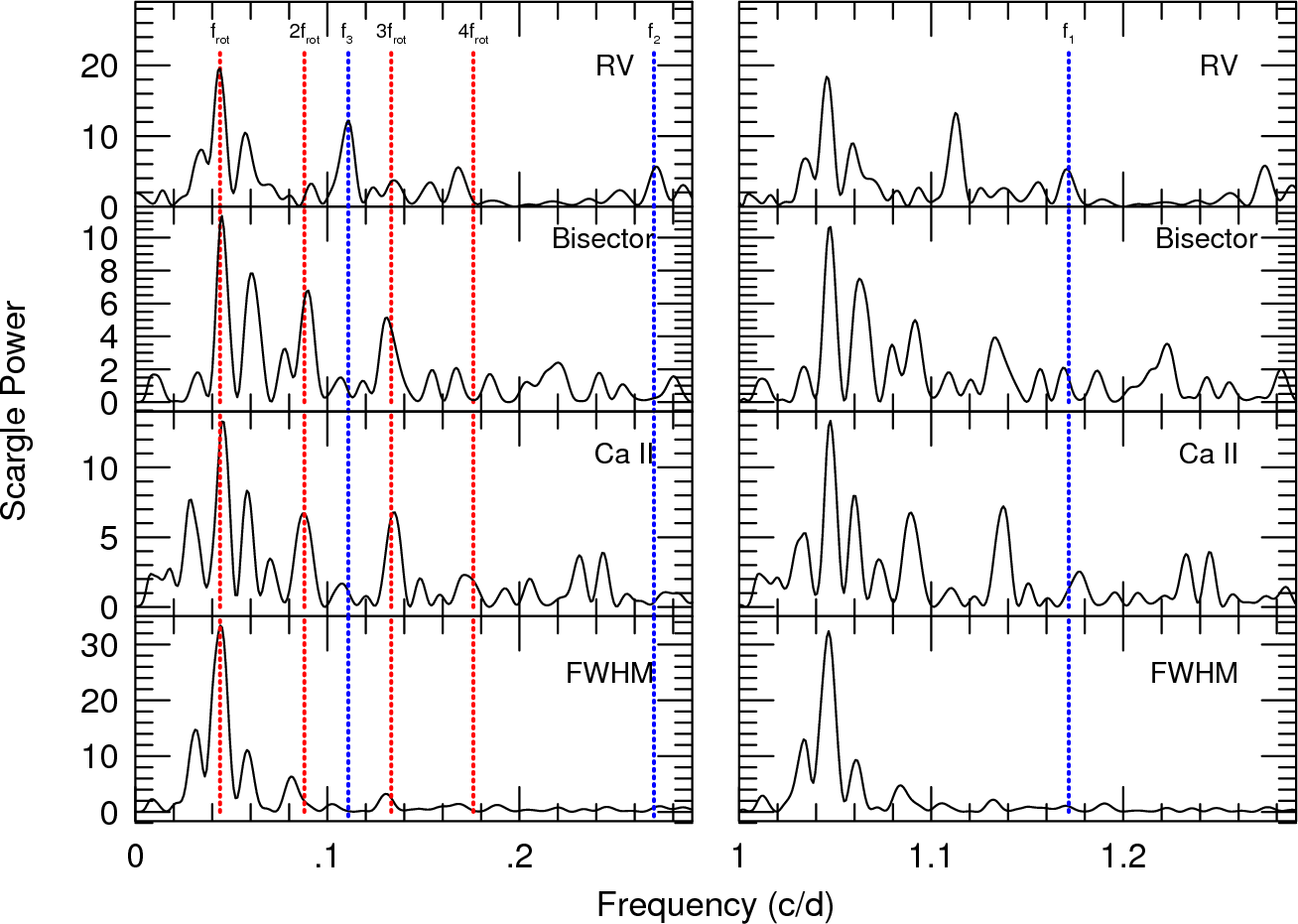
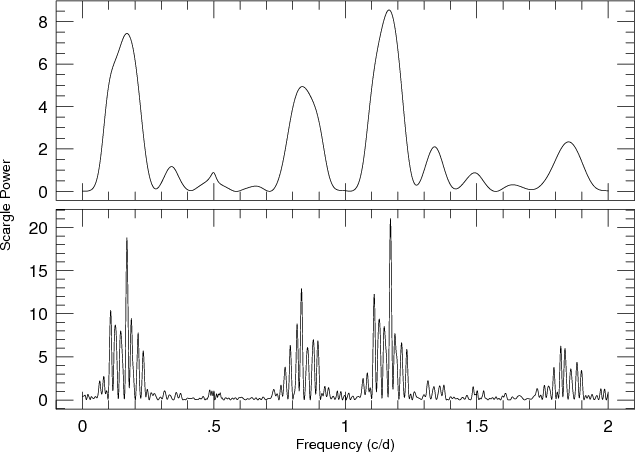
Figure 1: Scargle periodograms of the RV ( top), bisector ( upper middle), Ca II S-index ( lower middle), and FWHM ( bottom) measurements for the frequency range 0-0.3 c d-1 ( left panels) and 1.0-1.3 c d-1 ( right panels). The vertical blue lines mark frequencies seen only in the RV (the one in the right panel is the transit frequency). Vertical red lines mark the rotational frequency and its first 3 harmonics. |
| Open with DEXTER | |
- to assess the statistical significance of CoRoT-7b seen in the RV data;
- to look for possible additional planet signals in the HARPS data;
- to understand the nature of all detected signals in the HARPS RV data;
- to obtain the best possible determination of the mass, and thus density of CoRoT-7b.
2 Observations
The HARPS spectrograph obtained 106 RV measurements for CoRoT-7 over a time span of 4 months. We refer the reader to Q09 for a detailed description of the RV measurements. Besides RV information, the HARPS data also provided information on the activity of the star via the bisector span of the cross correlation function (CCF), the Ca II S-index, and the full-width at half maximum (FWHM) of the CCF. In particular, the line bisector has become a common tool for confirming exoplanet discoveries (e.g. Hatzes et al. 1988; Queloz et al. 2001). Figure 1 of Q09 shows the RV measurements for CoRoT-7 as well as the activity indicators.
3 Scargle periodograms of measured quantities
A periodogram analysis can give us a quick overview as to possible periods
that may be present in the data.
Scargle periodograms were calculated for the four quantities measured
from the HARPS spectra: RV, bisector span,
Ca II S-index, and the FWHM of the CCF.
These are shown in Fig. 1. The RV measurements
contain information about possible planetary companions and activity
while the other quantities should only contain information
on stellar activity. A comparison of the periodograms gives a first indication
as to which peaks in the RV periodogram arise from
activity and those which may be due to companions.
Two frequency ranges are shown. The left panels are for
![]() c d-1 and the right panels are for
c d-1 and the right panels are for
![]() c d-1. The vertical blue lines indicate RV
frequencies not seen in the activity indicators. The one in the right panel
is the CoRoT-7b transit frequency. Because of 1-day aliases all frequencies
in the left panel also appear as peaks at
c d-1. The vertical blue lines indicate RV
frequencies not seen in the activity indicators. The one in the right panel
is the CoRoT-7b transit frequency. Because of 1-day aliases all frequencies
in the left panel also appear as peaks at ![]() in the right panel.
(Note: we have not marked the 1-day alias of the CoRoT transit frequency
at 0.17 c d-1, although one can see a peak at this frequency location.)
The vertical red lines mark the
rotational frequency,
in the right panel.
(Note: we have not marked the 1-day alias of the CoRoT transit frequency
at 0.17 c d-1, although one can see a peak at this frequency location.)
The vertical red lines mark the
rotational frequency,
![]() ,
and its first 3 harmonics (2
,
and its first 3 harmonics (2
![]() ,
3
,
3
![]() ,
and 4
,
and 4
![]() ).
).
There are several important features to note in these periodograms. First,
the dominant peak in all 3 quantities occurs at
![]() c d-1,
the rotational frequency as determined from the CoRoT light curve.
Clearly, RV variations are dominated by the activity
RV jitter from rotational modulation which will complicate the extraction
of RV variations due to bona fide companions.
Second, the periodograms of the bisectors and
Ca II look remarkably similar with the same peaks identifiable in both periodograms.
Third, although the FWHM periodogram shows similar peaks near the
rotational frequency, its shape looks more like the RV periodogram
but without the peaks shown by the vertical dashed lines. The
strong peaks at
c d-1,
the rotational frequency as determined from the CoRoT light curve.
Clearly, RV variations are dominated by the activity
RV jitter from rotational modulation which will complicate the extraction
of RV variations due to bona fide companions.
Second, the periodograms of the bisectors and
Ca II look remarkably similar with the same peaks identifiable in both periodograms.
Third, although the FWHM periodogram shows similar peaks near the
rotational frequency, its shape looks more like the RV periodogram
but without the peaks shown by the vertical dashed lines. The
strong peaks at
![]() and 0.13 c d-1, which are the first
and second harmonics of
and 0.13 c d-1, which are the first
and second harmonics of
![]() ,
are not as strong in the FWHM as in the
bisector and Ca II periodogram.
The most important point is that the
3 peaks seen in the RV data at
,
are not as strong in the FWHM as in the
bisector and Ca II periodogram.
The most important point is that the
3 peaks seen in the RV data at
![]() ,
0.27, and 1.17 c d-1 (and their 1-day aliases) are not found in any of the other
quantities. This is our first hint for the presence of RV variability not
associated with
stellar activity.
,
0.27, and 1.17 c d-1 (and their 1-day aliases) are not found in any of the other
quantities. This is our first hint for the presence of RV variability not
associated with
stellar activity.
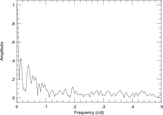
Figure 2 shows the spectral window for the data. As expected it is rather complex with strong sidelobes at +0.013 and 0.04 c d-1. Note that the same spectral window applies for all data (RV, bisectors, Ca II, and FWHM).
4 Frequency analysis of the data sets
It is evident from the periodograms that all spectral quantities have multi-periodic variations. As such they are well suited to the classic technique of pre-whitening often employed in the study of stellar oscillations. In this process a Fourier transform (FT) finds the highest peak in the power spectrum. A least squares fit to the frequency, amplitude, and phase to the found signal is made and then subtracted from the time series. Note that by subtracting this signal we also remove all aliases of the dominant frequency. A subsequent FT on the residuals yields the next dominant frequency in the time series. This sequential subtraction of dominant components is continued until the level of the noise is obtained using the criterion that peaks more than 4 times the Fourier noise level are regarded as real (Kuschnig et al. 1997). This frequency analysis was performed on the HARPS data using the program Period04 (Lenz & Breger 2004).
4.1 Radial velocity data
A pre-whitening analysis of the RV measurements was already presented in Q09. In that analysis a 12-component sine fit was made to the data which resulted in an rms to the fit of 1.81 m s-1. Table 1 lists frequencies using a more conservative solution. In this case the stopping criterion for the pre-whitening (last significant peak) was assessed using a bootstrap randomization procedure (e.g. Kürster et al. 1997). Frequencies above the horizontal line have a false alarm probability less than or equal to about 1%. The rms scatter of the fit to the RV is 2.96 m s-1 which is significantly higher than the mean RV error of 1.89 m s-1. Including the two frequencies below the space break results in an rms scatter of 2.18 m s-1, only slightly worse than the 12-component fit from Q09. Figure 5 in Q09 shows the fit to the RV data provided by the 12-component fit. The 9-component fit listed in Table 1 is of comparable quality so is not shown here.
Most of the frequencies from the FT analysis arise from stellar activity
with the most dominant one being the rotational frequency,
![]() c d-1 and its harmonics. This is noted in the comment column.
The rotational period derived from the RV data is 22.32
c d-1 and its harmonics. This is noted in the comment column.
The rotational period derived from the RV data is 22.32 ![]() 0.08 days,
hence larger than the value of 21.65
0.08 days,
hence larger than the value of 21.65 ![]() 0.03 days obtained from the CoRoT
light curve.
It is not known whether this
difference merely reflects the difficulty in measuring the rotational period
from such complex RV and light curves, or if this is a real difference
due to possibly differential rotation.
There are 3 frequencies denoted f1, f2, and f3 that are not readily
associated with stellar activity. The frequency f1 is the CoRoT-7b transit
frequency of 1.17165 c d-1, f2 is the 3.7-day planet reported
by Q09, and f3 corresponds to a period of 9.02 days and will discussed at
length below.
In Table 1 there are three additional frequencies above the space break and
two below that could not be readily associated
with rotational harmonics, but as we show below these are most likely
related to the activity signal. For convenience in referencing we denote
sequentially the additional frequencies f4 - f8, although
for the following discussion f1, f2, and f3 are the most important.
0.03 days obtained from the CoRoT
light curve.
It is not known whether this
difference merely reflects the difficulty in measuring the rotational period
from such complex RV and light curves, or if this is a real difference
due to possibly differential rotation.
There are 3 frequencies denoted f1, f2, and f3 that are not readily
associated with stellar activity. The frequency f1 is the CoRoT-7b transit
frequency of 1.17165 c d-1, f2 is the 3.7-day planet reported
by Q09, and f3 corresponds to a period of 9.02 days and will discussed at
length below.
In Table 1 there are three additional frequencies above the space break and
two below that could not be readily associated
with rotational harmonics, but as we show below these are most likely
related to the activity signal. For convenience in referencing we denote
sequentially the additional frequencies f4 - f8, although
for the following discussion f1, f2, and f3 are the most important.
|
Figure 2: Spectral window function for the HARPS measurements. |
| Open with DEXTER | |
Table 1: Frequencies and amplitudes found by a pre-whitening procedure on the HARPS RV data.
The CoRoT light curve for CoRoT-7 is complex and shows evidence for spot evolution on time scales of less than 150 days, or comparable to the time span of our RV measurements. Although the fit to the data using the full RV data set is excellent, the Fourier sine components may not accurately represent the activity variations over such a long time span. An analysis of the data in subsets of shorter time interval may minimize the uncertainties in the activity signal due to spot evolution.
To minimize possible effects of spot evolution, a frequency analysis was also performed on sub-sections of the HARPS data. The RV data were divided into 3 sets each roughly spanning one rotation period. The time span of these data sets are listed in the first 3 lines of Table 2. When analyzing data containing periods comparable to the time span of the data string there can be risks to using the pre-whitening procedure. This is certainly true for the rotational period and to some extent to the 9-d period since it only undergoes 2 cycles over the time span of the subset observations. Likewise the 0.85-d suffers from being severely under-sampled for some of the data subsets. In short, alias effects and spectral leakage may result in a spurious period being identified and removed from the data and thus resulting in an erroneous solution.
Indeed, when performing a straight pre-whitening procedure to Subset 1 the dominant
frequency is f = 0.13 c d-1 and the rotational frequency appears
at 0.05 c d-1. Only f2 is recovered. However, when one first
fits the data using the CoRoT-7b frequency first, the procedure recovers
both f2 and f3. A pre-whitening analysis on Subset 2 recovers
![]() ,
f1, and f2, but the nearest frequency to f3 was at 0.08 c d-1.
Subset 3 also yields different results. The dominant frequency occurs at 0.03 c d-1,
significantly different from
,
f1, and f2, but the nearest frequency to f3 was at 0.08 c d-1.
Subset 3 also yields different results. The dominant frequency occurs at 0.03 c d-1,
significantly different from
![]() .
Both f2 and f3 are recovered, but the nearest frequency
to f1, the transit frequency, is at 1.18 c d-1.
.
Both f2 and f3 are recovered, but the nearest frequency
to f1, the transit frequency, is at 1.18 c d-1.
Therefore, in fitting the subset
data we assumed that f1, f2, and f3 were present in the data
asked the question ``Can the subset
data be fit using these frequencies?'' To answer this we first
fit and removed the frequencies that were found in the full data set,
namely
![]() ,
f1, f2, and f3. In this fitting only the frequencies were
held fixed, but the amplitudes and phases were allowed to vary. The pre-whitening
procedure was continued until the rms fit to the data was comparable to the HARPS
measurement error (better than 2 m s-1).
,
f1, f2, and f3. In this fitting only the frequencies were
held fixed, but the amplitudes and phases were allowed to vary. The pre-whitening
procedure was continued until the rms fit to the data was comparable to the HARPS
measurement error (better than 2 m s-1).
Tables 3-5 lists the frequencies and amplitudes
from the Fourier analysis. In all cases the rms fit of the data is comparable
to the mean error of the HARPS measurements.
The amplitude of the
![]() ,
0.27, and 1.17 c d-1 signals remain relatively constant.
The largest amplitude variations are found for the frequency associated
with rotation, but it is not clear how significant these are given the
data sub-interval spans only one rotation period. The amplitude is thus
probably not well determined. In summary, this has established
that the RV variations in the subset data are consistent with the
presence of f1, f2, and f3, and with amplitudes comparable to those
found in the full data set. Note that the additional frequencies found in the
pre-whitening procedure can be identified with frequencies found in the full
data set analysis.
,
0.27, and 1.17 c d-1 signals remain relatively constant.
The largest amplitude variations are found for the frequency associated
with rotation, but it is not clear how significant these are given the
data sub-interval spans only one rotation period. The amplitude is thus
probably not well determined. In summary, this has established
that the RV variations in the subset data are consistent with the
presence of f1, f2, and f3, and with amplitudes comparable to those
found in the full data set. Note that the additional frequencies found in the
pre-whitening procedure can be identified with frequencies found in the full
data set analysis.
The referee suggested an analysis of the longest data string between
JD
= 2 454 847.6-2 454 884.7 as this has few gaps (Subset 4). A Fourier pre-whitening
procedure found f1 and f2, but was unable to find f3. This was also
the case when
we generated a fake data set using the periods listed in Table 1, sampled
in the same manner as Subset 4, and with random noise with
![]() m s-1. The pre-whitening procedure was also unable to detect f3even though it was present in the data. Table 6 lists the results of
the Fourier analysis by first fitting
m s-1. The pre-whitening procedure was also unable to detect f3even though it was present in the data. Table 6 lists the results of
the Fourier analysis by first fitting
![]() ,
f1, f2, and f3- similar to the procedure used for generating Tables 3-5. Note that the
amplitude of f3 is considerably lower than was found for Subsets 1-3.
This may be an indication that it is an artifact of the activity signal.
However, when performing the same analysis on the fake data generated
using the frequencies and amplitudes in Table 1 (again with
the appropriate sampling and noise), the fitted amplitude for
f3 is a factor of 3 less. The fitted amplitudes for the fake data
are listed in the third column of Table 6.
So, any evidence for amplitude variations
for f3 is inconclusive.
,
f1, f2, and f3- similar to the procedure used for generating Tables 3-5. Note that the
amplitude of f3 is considerably lower than was found for Subsets 1-3.
This may be an indication that it is an artifact of the activity signal.
However, when performing the same analysis on the fake data generated
using the frequencies and amplitudes in Table 1 (again with
the appropriate sampling and noise), the fitted amplitude for
f3 is a factor of 3 less. The fitted amplitudes for the fake data
are listed in the third column of Table 6.
So, any evidence for amplitude variations
for f3 is inconclusive.
Table 2: The data subsets.
Table 3: Frequencies found in data Subset 1.
Table 4: Frequencies found in data Subset 2.
Table 5: Frequencies found in data Subset 3.
Table 6:
Frequencies found in data Subset 4 using the same
analysis as Tables 3-5, i.e. first removing the contribution of
![]() ,
f1, f2, f3. Column 3 shows the amplitude
derived using fake data (see text).
,
f1, f2, f3. Column 3 shows the amplitude
derived using fake data (see text).
4.2 Frequency analysis of activity indicators
A Fourier analysis with pre-whitening
was performed on the bisector, Ca II S-index, and FWHM
measurements. These are listed in Tables 7-9.
The pre-whitening procedure was continued beyond the last frequency
we considered significant
to see if at any point a frequency was detected that coincided
with either f1, f2, and f3.
Both the bisector and FWHM measurements show frequencies near
f2:
![]() c d-1 (P = 3.6 d), but only after
pre-whitening the data well past our stopping criterion
(7th frequency found in the bisector and the 6th frequency
in the FWHM). These amplitude frequencies are essentially at or below the noise level.
Furthermore, when
we phase the bisector and FWHM data after removing all components except those
near the 3.7-d period, no obvious sinusoidal variations are present. We therefore
do not consider these frequencies to be significant.
c d-1 (P = 3.6 d), but only after
pre-whitening the data well past our stopping criterion
(7th frequency found in the bisector and the 6th frequency
in the FWHM). These amplitude frequencies are essentially at or below the noise level.
Furthermore, when
we phase the bisector and FWHM data after removing all components except those
near the 3.7-d period, no obvious sinusoidal variations are present. We therefore
do not consider these frequencies to be significant.
Table 7: Frequencies found in the bisector data using a pre-whitening procedure.
Table 8: Frequencies found in the Ca II data using a pre-whitening procedure.
Table 9: Frequencies found in the FWHM data using a pre-whitening procedure.
5 Statistical significance of the RV frequencies
A common way of assessing the statistical significance of a period found
in time series data is via the Scargle periodogram (Scargle 1982). In this formulation
of the Fourier transform the power of a peak is related to a statistical
significance rather than the amplitude of the periodic signal. If
a peak in the Scargle periodogram has power, z, then the false alarm
probability (FAP, probability that it is due to noise) can be calculated under
two cases. The first is if one is searching for an unknown signal
over a wide frequency range, and the second is for a period known to be
present in the data. In the former, the FAP is given by
FAP
![]() )
)
![]() ,
where N is the number of independent
frequencies. For the latter, the FAP is given by FAP
,
where N is the number of independent
frequencies. For the latter, the FAP is given by FAP
![]() ,
where now there is only one independent frequency (N=1).
,
where now there is only one independent frequency (N=1).
5.1 Statistical significance of 0.85-d RV period
Because we know that a 1.1716 c d-1 signal is present in the CoRoT light
curves we should ask: what is the FAP for a signal
at the known frequency of the CoRoT transit? Table 10
lists the Scargle power, z, and the false alarm
probability, FAP =
![]() for the peak at 1.17 c d-1 in each of the
data sets. Clearly, the
0.85-d period in the RV data is significant, whereas the false alarm probability of the
corresponding peak at the same frequency in any of the activity indicators
is over a factor of 20 higher.
for the peak at 1.17 c d-1 in each of the
data sets. Clearly, the
0.85-d period in the RV data is significant, whereas the false alarm probability of the
corresponding peak at the same frequency in any of the activity indicators
is over a factor of 20 higher.
Of course, the Scargle prescription uses the rms scatter of the full data set to set the noise level in assessing the FAP. If there is real variablity in the data this increases the rms scatter and results in an over-estimate of the FAP. For weaker signals in time series that are dominated by a stronger one, you should subtract the contribution of the dominant signal to get a better estimate of the FAP for the weaker signal.
Table 10: Scargle power and False Alarm Probability for the Peak at 1.17 c d-1, for RV, bisector, and Ca II data.

|
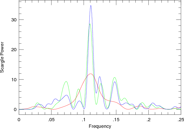
Figure 3: Scargle periodograms resulting from sequential adding of data subsets. Red line: subset 1, green line: subset 1 plus subset 2, blue: all data sets. |
| Open with DEXTER | |
Figure 3 shows the Scargle periodogram of the RV residuals after
subtracting all sine components except that due to the
CoRoT planet at 0.85 days.
The red line
shows the Scargle periodogram
using Subset 1, the green is after adding Subset 2, and the blue is
the periodogram of the full data set. The fact that the Scargle power increases
with the addition of each new data set (i.e. increasing statistical
significance) gives us some reassurance that the signal is indeed present
in all data sets. The final Scargle power of the 1.171 c d-1 signal is
z = 39, which results in an FAP of ![]() 10-17 for
a known signal in the data.
The FAP that noise would
create a peak with power higher anywhere in the full spectral
range (first equation from above)
is
10-17 for
a known signal in the data.
The FAP that noise would
create a peak with power higher anywhere in the full spectral
range (first equation from above)
is ![]() 10-15. Thus
this signal would be highly significant even if
we were unaware of the CoRoT transit period.
10-15. Thus
this signal would be highly significant even if
we were unaware of the CoRoT transit period.
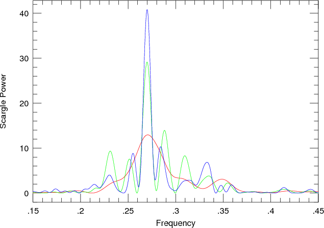
5.2 Statistical significance of 3.7-d RV period
The 3.7-d period ( f2 = 0.11 c d-1) has Scargle power of 5.67. Based on this power level we would normally not be considered the signal to be significant. An FAP was assessed by using a bootstrap randomization method. The RV values of the data (with all signals present) were shuffled randomly keeping the observation times fixed and a periodogram calculated for this random data. After 105 such ``shuffles'' the number of random periodograms having power greater than 5.67 over the frequency range 0-0.5 d-1 gave an estimate of the FAP. This value was 0.3.
However, as stated earlier, this FAP may be overestimated due to the
presence of the other signals in the RV data. To get a more realistic
assessment of the false alarm probability the
contributions from all sine components except that due to the
3.7-day period were subtracted from the three subsets
(the 3.7-d residuals).
Figure 4 shows the Scargle
periodogram after sequentially adding the residual RVs from each
of the data subsets.
The Scargle power increases with the addition of each subset and the
final value is 40 which corresponds to an FAP ![]() 10-16.
10-16.
5.3 Statistical significance of 9.0-d RV period
The peak at 9 days in the RV periodogram has Scargle power of 12.13.
A bootstrap randomization with 105 shuffles yields an FAP
![]() .
We can be confident that this signal is
statistically significant even without subtraction of the other signals.
Figure 5 shows the Scargle periodograms for the 9-d RV residuals, i.e. the
RV measurements with all signals except the 9-d period subtracted, and
as each subset is added. The increase in the statistical significance
with the addition of more RV measurements is an indication of a
long-lived and coherent signal. The FAP of the final peak after including
all RV measurements is
.
We can be confident that this signal is
statistically significant even without subtraction of the other signals.
Figure 5 shows the Scargle periodograms for the 9-d RV residuals, i.e. the
RV measurements with all signals except the 9-d period subtracted, and
as each subset is added. The increase in the statistical significance
with the addition of more RV measurements is an indication of a
long-lived and coherent signal. The FAP of the final peak after including
all RV measurements is ![]() 10-16.
10-16.
|
Figure 4: Scargle periodograms resulting from sequential adding of residual RV data for the 3.7-day period. Red line: subset 1, green line: subset 1 plus subset 2, blue: all data sets. All sine components except the that associated with the 9.02-day period. |
| Open with DEXTER | |
|
Figure 5: Scargle periodograms resulting from sequential adding of residual RV subsets for the 9-day period. Red line: subset 1, green line: subset 1 plus subset 2, blue: all data sets. |
| Open with DEXTER | |
6 Is the 0.85-d period an alias of a rotation harmonic?
The Scargle periodograms in Fig. 1 are
dominated by the rotational frequency,
![]() .
However, there is also power at the first
two harmonics of the rotational frequency, namely 2
.
However, there is also power at the first
two harmonics of the rotational frequency, namely 2
![]() and
and
![]() .
Indeed, Q09 applied harmonic filtering using
the rotational frequency and its first two harmonics to remove the signature of activity. Because of this there
is some concern that the 1.1715 transit frequency is close to the one-day alias of the 3rd harmonic
of the rotational frequency (i.e.
.
Indeed, Q09 applied harmonic filtering using
the rotational frequency and its first two harmonics to remove the signature of activity. Because of this there
is some concern that the 1.1715 transit frequency is close to the one-day alias of the 3rd harmonic
of the rotational frequency (i.e.
![]() c d-1). In the best case, the activity signal can thus contribute
some power at the orbital frequency of CoRoT-7b.
In the worse case all the RV signal at this frequency could arise from
activity.
c d-1). In the best case, the activity signal can thus contribute
some power at the orbital frequency of CoRoT-7b.
In the worse case all the RV signal at this frequency could arise from
activity.
Q09 argued that because repeated measurements were taken on the same nights, that this alias effect was minimized and that the 0.85-d RV period was the one actually present in the data. To investigate whether alias effects of a rotational harmonic can account for the observed 0.85-d period in the RV data we performed an analysis on a subset of the RV consisting only of those nights for which at least 3 RV measurements were made during the night. In the following analysis it is assumed that the activity signal contributes a constant value to the measured RV on a given night. This is a reasonable assumption. The maximum time separation between the first and last measurement on a given night is less than 4 h. This corresponds to a change in rotation phase of only 0.007. The contribution of stellar activity to the measured RV should thus be a constant over that time. This also assumes that spot evolution over 4 h is negligible. Meanwhile, the change in orbital phase of CoRoT-7b is 0.2 and should cause the dominant variations observed in the RV during the course of the night.
It is not strictly true that the non-CoRoT-7b RV variations are constant during the night. The orbital motion due to the CoRoT-7c should produce an appreciable variation over 4 hours. However, this contribution is also relatively small. Over 4 hour time span the orbital phase of CoRoT-7c only changes by 0.05 which corresponds to a maximum RV variation of only 1.5 m s-1 well below the measurement error.
There were 7 nights where at least 3 RV measurements of CoRoT-7 were made resulting in a total of 21 measurements. The data from these nights were treated as 7 independent data sets with each one have a different a zero-point velocity which could vary from night to night. A least squares sine-fit the 7 data sets was made keeping the period fixed to the transit period of 0.8535 days, but allowing phase and the zero-point value for each night to vary. The advantage of such an approach is that it is a ``minimal impact'', low pass filter that makes no assumptions about the underlying time variability due to stellar activity, only that it is constant on a given night.
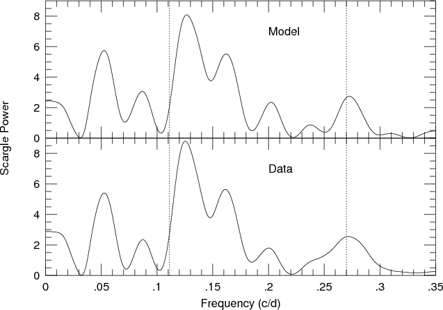
The top panel of Fig. 6 shows the
Scargle periodogram of these 21 RV measurements after
subtracting the individual zero-point offsets determined by the least squares fitting. The
strongest peak is at the transit frequency of 1.1715 c d-1 and
with a smaller peak at the
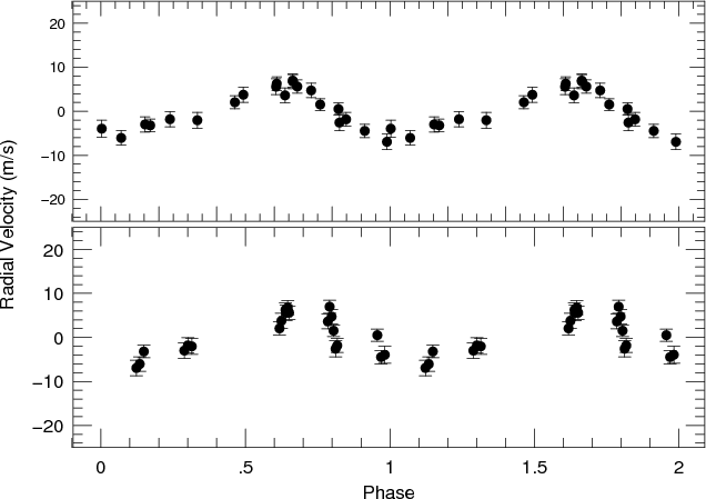
alias frequency of 0.1715 c d-1. Figure 7
shows the RV measurements
phased to the period of CoRoT-7b and the alias period (5.7 days). The ``cleaner'' phase diagram
of the 0.85 d period supports that this is the true period in the data, and not the alias of
![]() .
.
The false alarm probablity of the peak at 1.1715 c d-1 was
assessed using a bootstrap randomization procedure. The RV values were shuffled
![]() times keeping the observed times fixed and periodograms calculated
for this random data. Over the frequency range
times keeping the observed times fixed and periodograms calculated
for this random data. Over the frequency range
![]() c d-1there was only four instances
where the periodogram of the random exceeded the power of the real data.
The FAP for this signal is thus
c d-1there was only four instances
where the periodogram of the random exceeded the power of the real data.
The FAP for this signal is thus ![]()
![]() .
We should note that this
bootstrap was evaluated over the full frequency range 0-2 c d-1.
Since we are interested in the known frequency of CoRoT-7c it is more
appropriate to evaluate the bootstrap
over a much narrower range centered on
.
We should note that this
bootstrap was evaluated over the full frequency range 0-2 c d-1.
Since we are interested in the known frequency of CoRoT-7c it is more
appropriate to evaluate the bootstrap
over a much narrower range centered on
![]() c d-1. The FAP of this signal is almost certainly much less.
c d-1. The FAP of this signal is almost certainly much less.
|
Figure 6: (Top) Scargle periodogram of the data set consisting of 7 nights where at least 3 RV measurements were made. The measurements from each night were considered an independent data set and a fit was made using the period of CoRoT-7b and allowing zero point offset from each night to vary. The periodogram is of the data with the offset to each night subtracted. (Bottom) Same as in the top panel but with the addition of 16 nights for which two RV measurements were made per night. |
| Open with DEXTER | |
There were an additional 16 nights where 2 RV measurements were taken
of CoRoT-7. The time separation of these points are large enough to provide
some good sampling of the 0.85-d sine wave presumed to be in the data.
These nights were added to the data subset of 3 points per night
to give a total of 53 data points spread over 23 nights.
A new fit was performed, again allowing the
nightly zero-point values to vary, but keeping the period fixed to the transit period.
The lower panel of Fig. 6
shows the periodogram of these data with the zero point offsets applied. Note
that the Scargle power has significantly increased indicating a more signficant
detection (FAP ![]() 10-16). Also, the frequency at
1.1716 c d-1 is still higher than the alias frequency. A phase diagram
of these data will be shown below when we present orbital solutions.
10-16). Also, the frequency at
1.1716 c d-1 is still higher than the alias frequency. A phase diagram
of these data will be shown below when we present orbital solutions.
|
Figure 7: (Top) RV measurments of the 7-night data set (zero-point offsets applied) phased to the period of CoRoT-7b. (Bottom) same measurements phased to the alias period of 5.82 days. |
| Open with DEXTER | |
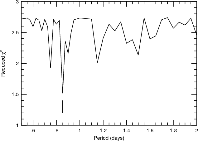
We also investigated whether the period of CoRoT-7b could be extracted from the
data without a priori knowledge of the transit period.
To do this a range of periods
were fit to the 53 RV measurements of the data set with
multiple observations per night. At each trial fit the period was fixed, but the phase and
zero-point offset were allowed to vary. Figure 8 shows the reduced
![]() fit to the data as a function of the fitting period. Good fits
occur at
periods where
fit to the data as a function of the fitting period. Good fits
occur at
periods where ![]() is minimized. This procedure could be considered as a variant
of the phase dispersion minimization technique of Stellingwerf (1978), but
which allows the mean value of
individual data sets to float (i.e. a ``floating mean'' phase dispersion minimization). The
deepest
is minimized. This procedure could be considered as a variant
of the phase dispersion minimization technique of Stellingwerf (1978), but
which allows the mean value of
individual data sets to float (i.e. a ``floating mean'' phase dispersion minimization). The
deepest ![]() minimum is near the period of CoRoT-7b (vertical line).
Other minima are clearly alias periods and phasing of the data to these periods
does not produce as clean a phase diagram as for the CoRoT-7b period.
minimum is near the period of CoRoT-7b (vertical line).
Other minima are clearly alias periods and phasing of the data to these periods
does not produce as clean a phase diagram as for the CoRoT-7b period.
6.1 Fourier analysis of nightly offsets
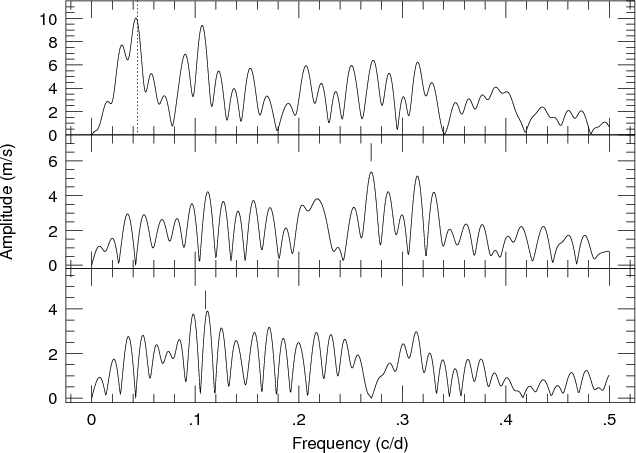
As a sanity check we performed a Fourier analysis on the nightly offsets produced by our least squares fitting. If these derived nightly offsets have some relationship to the activity we should see evidence of the rotational period. The top panel of Fig. 9 shows the Fourier transform of the nighty offsets (23 values). The highest peak corresponds to the rotational frequency of CoRoT-7 (indicated by the vertical dashed line). This indicates that the nightly zero-point offset indeed follows the RV rotational modulation due to activity.
Of interest is when we pre-whiten the nightly offsets to search for additional periods. The second panel shows the offset data after removing the contribution of the rotational frequency. The highest peak corresponds to a frequency of 0.27 c d-1 (indicated by the vertical line). The bottom panel shows the amplitude spectrum of the residuals after removing the contribution of the 0.27 c d-1 frequency. The highest peak corresponds to 0.112 c d-1, close to the 0.11 c d-1 frequency found in the RV (indicated by the vertical line). It is reassuring that the nightly offsets show evidence for the rotation period of the star, but also the 3.7-d and 9-d period found in the RV analysis.
|
Figure 8:
The reduced |
| Open with DEXTER | |
|
Figure 9: A pre-whitening on the zero-point offsets of the multi-measurement nights found by the least squares fitting. ( Top) Amplitude spectrum of the zero-point values. The dashed line indicates the rotation period of CoRoT-7b. ( Middle) The amplitude spectrum after removing the rotational frequency. The vertical line corresponds the frequency of the 3.7-d period of CoRoT-7c. ( Bottom) The amplitude spectrum after also removing 3.7-d period signal. The vertical line corresponds to the frequency f3. |
| Open with DEXTER | |
7 On the nature of the 9-d period
|
Figure 10:
(Top) Scargle periodogram for the fit to RV first data subset (truncated JD = 4775-4807)
sampled in the same manner as the data and with noise at a level of
|
| Open with DEXTER | |
In Q09 the two approaches to the RV data analysis (harmonic filtering and
Fourier
pre-whitening) agree on the presence of a 0.85-d and 3.7-d period in the data.
The main difference to the two approaches was that the pre-whitening procedure
yielded a significant period at 9-d, whereas this signal was absent in the harmonic filtering of activity
signal. The obvious interpretation is that the 9-d period arises from the activity signal.
However, the harmonic filtering worked on sub-sets of the data that were roughly
the length of the rotation period, whereas the pre-whitening
procedure was performed on the full dataset.
The 9-d period is very close to
![]() ,
i.e.
the first harmonic of the rotation period. There is a danger that when applying
harmonic filtering one may remove real signals not associated with a rotational harmonic.
,
i.e.
the first harmonic of the rotation period. There is a danger that when applying
harmonic filtering one may remove real signals not associated with a rotational harmonic.
To test this hypothesis the frequency solution of the Subset 1 (Table 3)
was used
to generate a fake data set. This fake data included the signals f1, f2,
and f3.
The fits were sampled in exactly the same way as the real data and
noise at a level of
![]() m s-1 was also added. The Scargle periodogram of the
fake data (top panel) is compared to the periodograms of the real data
(lower panel) in Fig. 10. The frequency of the input
3.7-d and 9-d period signals are shown as vertical lines.
m s-1 was also added. The Scargle periodogram of the
fake data (top panel) is compared to the periodograms of the real data
(lower panel) in Fig. 10. The frequency of the input
3.7-d and 9-d period signals are shown as vertical lines.
There are two things to note about this figure. The periodogram of the fake data looks exactly like the real data, as it should. After all, the rms scatter about the fit is under 2 m s-1. If you fit the data you fit the periodogram. Note, however, because of the short data window the true frequency in the data, f3, appears at a slightly different frequency of 0.12 c d-1.
This fake Subset 1 data set was analyzed using harmonic analysis
and pre-whitening. The data was first fit using the rotational frequency
and its first two harmonics (
![]() ,
2
,
2
![]() ,
and 3
,
and 3
![]() )
as well
as 0.5
)
as well
as 0.5
![]() (there was evidence for the presence of this frequency,
see Table 1). The frequencies were kept fixed, but the amplitude and phase
were made to vary. The pre-whitening procedure was then carried out to
find additional frequencies. The results are listed in Table 11. The
pre-whitening procedure found only 2 additional frequencies, f1 and
f2, but not f3 even though it was present in this fake data.
The same result was found when applying this procedure to the other
data sets.
(there was evidence for the presence of this frequency,
see Table 1). The frequencies were kept fixed, but the amplitude and phase
were made to vary. The pre-whitening procedure was then carried out to
find additional frequencies. The results are listed in Table 11. The
pre-whitening procedure found only 2 additional frequencies, f1 and
f2, but not f3 even though it was present in this fake data.
The same result was found when applying this procedure to the other
data sets.
Harmonic filtering was also performed on the full RV (real) data set
by first fitting
![]() ,
2
,
2
![]() ,
and 3
,
and 3
![]() to the data and
then continuing the pre-whitening procedure to find additional frequencies.
After all frequencies were found the solution optimized by fitting all
components simultaneously.
The results are shown in
Table 12. The frequencies f1,
f2, and f3 were recovered in spite of the harmonic pre-filtering.
to the data and
then continuing the pre-whitening procedure to find additional frequencies.
After all frequencies were found the solution optimized by fitting all
components simultaneously.
The results are shown in
Table 12. The frequencies f1,
f2, and f3 were recovered in spite of the harmonic pre-filtering.
This investigation has demonstrated that one should be careful in filtering the time
series data using harmonics of the
rotational frequency of CoRoT-7 on a limited time span data set. In this case,
using rotational harmonics essentially filtered out the
real period that was in the simulated data.
When applying rotational harmonic
filtering to the full real data set the 9-d period was still recovered.
The reason for this is that over a 23-d time span there is
little difference between
![]() c d-1 and the first harmonic
of the rotational frequency,
c d-1 and the first harmonic
of the rotational frequency,
![]() c d-1. Harmonic filtering will essentially remove this signal. However,
over the 100 days that the RV data were acquired the subtle frequency difference
between f3 and 2
c d-1. Harmonic filtering will essentially remove this signal. However,
over the 100 days that the RV data were acquired the subtle frequency difference
between f3 and 2
![]() can be resolved and harmonic filtering cannot
fully remove the signal due to f3. When performing an analysis on data subsets
it is instructive to
look also at the full data covering the longest time span.
can be resolved and harmonic filtering cannot
fully remove the signal due to f3. When performing an analysis on data subsets
it is instructive to
look also at the full data covering the longest time span.
7.1 Bisector - RV correlations
Table 11: Frequencies found in the simulated data set of Subset 1 (Fig. 10) using a pre-whitening procedure and harmonic analysis.
Table 12: Pre-whitened frequencies found in the RV data after first fitting the rotational frequency and its first 2 harmonics.
The HARPS data also contain three indicators of activity: the FWHM of the CCF, the bisector of the CCF, and the Ca II emission measure. Of these 3 activity indicators only the line bisectors have a direct relationship to the RV variations due to activity. Ca II emission originates in plage and these regions do not necessarily have the same surface distribution as spots. For cool spots the FWHM is out-of-phase with the RV variations. The FWHM is a minimum when the spot distortions are the wings of the spectral line (i.e. limb of star) and a maximum when the spots are at disk center (zero RV). Thus there is a phase shift ofRV variations caused by cool spots should show an anti-correlation (negative slope) with the bisector variations (see Queloz et al. 2001). The RV variations of CoRoT-7 do show a slight anti-correlation with the bisectors (left panel of Fig. 11). If an RV signal is not due to activity, then removing this from the observed RV measurements should result in a stronger correlation between the bisectors and RV variations. Indeed, when one removes that signal of the 0.85-d, 3.7-d, and 9-d period from the RV data the bisector span - RV variations become more correlated (r = -0.42, right panel). This suggests that the 0.85-d, 3.7-d, and 9-d periods (i.e. f1, f2, and f3) found in the RV data are not associated with activity.
| Figure 11: (Left) Bisctor span of the CCF versus the RV measurements. The correlation coefficient is -0.28. (Right) The Bisector-RV correlation after f1, f2, f3 (planet signals) have been removed from the data. The correlation coefficient is -0.42. |
|
| Open with DEXTER | |
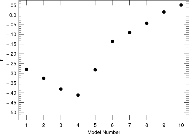
Figure 12 shows the correlation coefficient between the bisector and RV measurements as a function of data sets with the contributions of various frequencies removed (denoted ``Model Number'') Model 1 is to the original RV data set. Model 2 is this data set with the 0.85-d period removed. Model 3 is the previous model, but with the 3.7 d period also removed. Model 4 is the data set with the 0.85-d, 3.7-d, and 9-d periods removed. Note that the correlation coefficient becomes more negative with the removal of each data set suggesting that these 3 periods are not associated with stellar activity.
Model 5 represents Model 4 -
![]() .
Each subsequent model is the previous
model with
successive frequencies listed in Table 1 removed (and skipping of course
f1, f2, and f3 already subtracted in Model 4). The fact that the
RV-Bisector variations become more uncorrelated with
the removal of additional frequencies
suggests that all frequencies in Table 1 except f1, f2, and
f3 are most likely due
to activity.
.
Each subsequent model is the previous
model with
successive frequencies listed in Table 1 removed (and skipping of course
f1, f2, and f3 already subtracted in Model 4). The fact that the
RV-Bisector variations become more uncorrelated with
the removal of additional frequencies
suggests that all frequencies in Table 1 except f1, f2, and
f3 are most likely due
to activity.
|
Figure 12:
The correlation coefficient of the CCF bisector span with RV
as a function of different versions of the RV data with the
frequencies in Table 1 removed. Model 1: raw
data, Model 2: f1 removed, Model 3: f1 and f2 removed,
Model 4: f1, f2, and f3 removed. Model 5: Model 4 and
|
| Open with DEXTER | |
Because the RV variations are directly related to the bisector
variability we can use the temporal variations of the RV to produce
a predicted bisector variability. Saar & Donahue (1997) gave relationships
relating both the bisector span and RV amplitude as a function of spot filling
factor and rotational velocity of the star. The RV-to-Bisector amplitudes
ratio from their expressions is predicted to be about a factor of 10. However,
the exact ratio depends on several factors, primarily how one measures
the bisector span and which spectral lines are used. Their result cannot
be directly compared to the bisector measurements of the CCF from the HARPS
data.
A better way is to use the RV-to-Bisector amplitude
ratio estimated by comparing the amplitudes of
frequencies found in both the RV and bisector amplitude spectra and using data
where these quantities (bisector and RV) were measured in a consistent way.
The RV frequencies
![]() c d-1 and
0.094 c d-1 in Table 1 have amplitudes of 7.5 m s-1 and
5.69 m s-1. The corresponding frequencies in the bisector amplitude
spectrum
have amplitudes of 4.21 m s-1 and 2.81 m s-1, respectively.
This implies that the RV-to-Bisector amplitude is
c d-1 and
0.094 c d-1 in Table 1 have amplitudes of 7.5 m s-1 and
5.69 m s-1. The corresponding frequencies in the bisector amplitude
spectrum
have amplitudes of 4.21 m s-1 and 2.81 m s-1, respectively.
This implies that the RV-to-Bisector amplitude is ![]() 2.
2.
We created a model of the bisector variations based on the amplitude spectrum of the RV measurements. Two fake data sets of bisector variations were generated. The first used all the frequencies in Table 1, excluding f1, f2, and f3. All amplitudes in Table 1 were reduced by a factor 0.5 corresponding to the bisector-to-RV amplitude ratio. The sampling of this time series was the same as the actual data. The bisector variations have an rms scatter of 4.5 m s-1 after removal of the dominant frequencies. This was taken as the mean bisector error and random noise at this level was added to the fake bisector data. The second data set was similar to the first one, but the frequency f3 was present with the appropriately scaled amplitude (i.e. only f1 and f2 were removed).
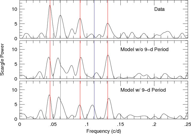
The top panel of Fig. 13 shows the Scargle periodogram of the actual bisector measurements. The middle panel shows the periodogram of the fake data, but without the presence of the 9-d period. The bottom panel shows the periodogram of the fake bisector data with the 9-d period present. Vertical red lines show the rotation frequency and its first 3 harmonics. The vertical blue line shows the frequency corresponding to the 9-d period.
There are two interesting features about this figure.
First, the periodogram of the
fake bisector data without the 9-d period looks qualitatively like the real data.
Many of the same peaks are seen in both periodograms.
The ratio of the amplitudes are not quite correct probably due to
the bisector data having more complicated noise characteristics than the
Gaussian noise in our simple model. Furthermore, for
high frequency components that the RV-to-Bisector amplitude ratio may be
different. The second important feature to note is that in the periodogram of the
fake data with the 9-d period present
there is a signficant peak at
![]() c d-1
that is not seen in the data periodogram. If the 9-d period was
due to activity we should have seen a
corresponding peak in the periodogram of the bisectors and most likely
in the Ca II and FWHM.
This also argues in favor
of the 9-d period not being related to activity.
c d-1
that is not seen in the data periodogram. If the 9-d period was
due to activity we should have seen a
corresponding peak in the periodogram of the bisectors and most likely
in the Ca II and FWHM.
This also argues in favor
of the 9-d period not being related to activity.
|
Figure 13: (Top) Scargle periodogram of the CCF bisector variations. (Middle) Scargle periodogram of a fit generated using the RV frequencies of Table 1, but without f1, f2, and f3present. Amplitudes were adjusted according to the measured RV-to-Bisector amplitudes. Random noise at the level observed for the bisector measurements were also added. (Bottom) Same as for the middle panel but with f3 (9-d period) present. |
| Open with DEXTER | |
8 A search for transits from CoRoT-7d
The CoRoT-7 light curve was analyzed to see if a 9-d transit signal could be found in the data. A similar investigation was already performed to search for transits from CoRoT-7c, but none was found (Q09). If the orbits of all planets are co-planar we do not expect to see transits from CoRoT-7d. However, if substantial differences of the orbital inclination between the planets exist, CoRoT-7d may well transit in spite of having a larger orbital radius than CoRoT-7c.
The CoRoT-7 light curve first had to be filtered for the large variations due to the stellar activity. This was done by: 1) normalizing the light curve by the maximum value; 2) performing outlier rejection; 3) reducing residual orbital effects by using a running median of length one orbit; and 4) tracking slow variations using a sliding polynomial of 12 hours and subtracting these. Finally, we fit the transit curve of CoRoT-7b and subtracted that from the light curve.
This processed light curve was then phase-folded to the 9.02 d period. No transit
signal above the noise was detected. We derive an upper limit of
![]() for the depth of any transit at a period of 9.02 d.
for the depth of any transit at a period of 9.02 d.
9 Orbital solutions
9.1 The 0.85-d period
Models of the internal structure of CoRoT-7b rely on the mass determination
which in turn hinges on the amplitude of the RV variations.
In Q09 the amplitude of CoRoT-7b was estimated to be 3.5 m s-1using two different approaches and this
corresponds to a planet mass of 4.8
![]() .
However, this value
was obtained after applying a correction term for the effects of the filtering
process to both techniques using simulated data.
The uncorrected pre-whitening
procedure amplitude was slightly higher at 4.2 m s-1 and
the harmonic filtering amplitude lower at 1.9 m s-1.
Clearly,
the amplitude of CoRoT-7b depends on how one removes the activity signal.
.
However, this value
was obtained after applying a correction term for the effects of the filtering
process to both techniques using simulated data.
The uncorrected pre-whitening
procedure amplitude was slightly higher at 4.2 m s-1 and
the harmonic filtering amplitude lower at 1.9 m s-1.
Clearly,
the amplitude of CoRoT-7b depends on how one removes the activity signal.
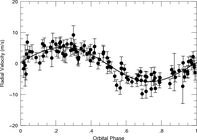
As an alternative approach to determining the RV amplitude of CoRoT-7b we took the results from Sect. 6. In this analysis we used only the RV data for which multiple measurements were made each night. A least squares sine fit to this data was made keeping the period fixed and allowing the nightly offset to vary. The final offsets were then subtracted from the individual nights and the data combined. This may be the best way to account for the RV variations of activity without any assumptions about its temporal behavior. An orbital solution was performed on all the residual RVs keeping the ephemeris, T0, fixed to the CoRoT transit time of 2 454 446.7311.
Table 13: Orbital parameters for the 0.85-d period.
Table 13 lists the orbital elements.
At first the nightly data were fit keeping the CoRoT transit period
of 0.8535 days. If we allow this parameter to vary we get a best fit to the
data with a period of 0.85359 days which is listed in the
table. Allowing the T0 to vary, but keeping the period fixed results
in T0 = 2 454 446.7330 a value very close to the CoRoT ephemeris.
Allowing the eccentricity to vary results in a best fit value of 0.08, but
with large error,
![]() 3.
We cannot exclude a slight eccentricity in the orbit, but given the
large variations due to activity and the additional companions, this may
be difficult to extract reliably from the RV data.
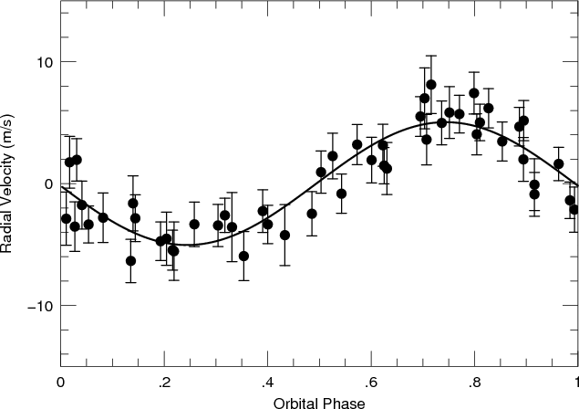
Figure 14 shows the zero-point corrected data phased to the
CoRoT transit ephemeris and a period of 0.85359. The solid line
represents the orbital solution.
3.
We cannot exclude a slight eccentricity in the orbit, but given the
large variations due to activity and the additional companions, this may
be difficult to extract reliably from the RV data.
Figure 14 shows the zero-point corrected data phased to the
CoRoT transit ephemeris and a period of 0.85359. The solid line
represents the orbital solution.
The derived K-amplitude is 5.04 ![]() 1.09 m s-1 which
results in a companion mass of 6.9
1.09 m s-1 which
results in a companion mass of 6.9 ![]() 1.4
1.4
![]() .
This is
slightly larger than the K-amplitude of 4.16
.
This is
slightly larger than the K-amplitude of 4.16 ![]() 0.27 m s-1(m = 5.75
0.27 m s-1(m = 5.75 ![]() 0.37
0.37
![]() )
by pre-whitening the full data set
(Q09). The K-amplitude from pre-whitening of the
full data set and the analysis of the subset RV data with
multiple measurements each night both suggest a slightly higher planet mass
than the 4.8
)
by pre-whitening the full data set
(Q09). The K-amplitude from pre-whitening of the
full data set and the analysis of the subset RV data with
multiple measurements each night both suggest a slightly higher planet mass
than the 4.8 ![]() 0.8
0.8
![]() of Q09, although all determinations
are consistent to within the errors.
of Q09, although all determinations
are consistent to within the errors.
|
Figure 14: (Top) Orbital solution for the 0.85-d period using the data with repeated nightly measurements and the appropriate zero-point offset applied. |
| Open with DEXTER | |
9.2 The 3.7-d period
RV residuals were produced by subtracting
all sine components except for f2 from the full RV data
set and an orbital solution calculated. In removing the
contribution of f1 the amplitude in Table 13 was used rather than the slightly higher
amplitude found in Table 1. The
derived amplitude is slightly lower than the one presented in Q09 (5.5 m s-1) that
removed f1 using the amplitude found in the pre-whitening procedure. In order to
estimate the range of velocity amplitudes for f2
a least squares fit to the original RV data was first made using
this frequency and the subsequent frequencies found in the
pre-whitening process sequentially subtracted. The range of amplitudes
for f2 during this
process ranged from 4.75 to 5.4 m s-1. An error of
![]() m s-1 was adopted which is
slightly more than the formal error of
m s-1 was adopted which is
slightly more than the formal error of
![]() m s-1 from the orbit fitting. Note that this formal error is much lower than for
the amplitude CoRoT-7b which was calculated using only a subset of the data.
m s-1 from the orbit fitting. Note that this formal error is much lower than for
the amplitude CoRoT-7b which was calculated using only a subset of the data.
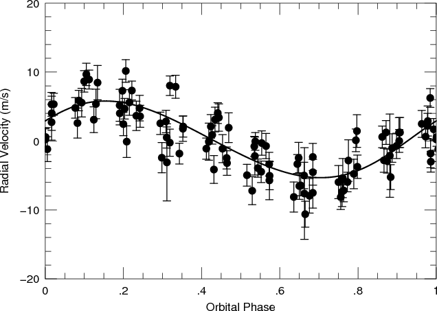
Figure 15 shows the orbital solution the 3.7-day period. The orbital elements are listed in Table 14. A slight eccentricity is found, but this may well be an artifact due to the filtering process.
|
Figure 15: The RV residuals of CoRoT-7 after removing all components in Table 1 except for f2 and phased to the 3.7 d period (points). The orbital fit is shown as a line |
| Open with DEXTER | |
9.3 The 9-d period
The RV residuals were calculated after subtracting all sine components in Table 1 except for f3 and again using the
amplitude for f1 from Table 13. The range of possible amplitudes for
f3 during the pre-whitening procedure was 5.5-7.15 m s-1.
We thus adopted an error in the ampitude of
![]() m s-1,
larger than the formal error of
m s-1,
larger than the formal error of
![]() m s-1, but probably a
more realistic estimate. A best fit orbit allowing the eccentricity
to vary resulted in a slightly negative value. We therefore took a solution with
the eccentricity fixed to zero with an error of
m s-1, but probably a
more realistic estimate. A best fit orbit allowing the eccentricity
to vary resulted in a slightly negative value. We therefore took a solution with
the eccentricity fixed to zero with an error of
![]() .
.
Figure 16 shows the orbital solution to the RV residuals using the 9-day period. The orbital elements are listed in Table 15. Note the gap-like structures in the phase curve. This is undoubtedly due to the period being nearly an integer value of one day, i.e. our typical sampling rate.
Table 14: Orbital parameters for the 3.7-d period.
10 On the dynamical stablity of the 3-planet system.
We also investigated whether the 3-planet system would be dynamically stable. Although a stable system is no proof that all 3 planets exist, an unstable system would indicate that the additional planetary signals found in the HARPS data may arise from activity.
10.1 An ultra-compact planet system?
The stability of planetary systems involves multiple interactions of planets by
mutual perturbations
often involving interactions of resonances between more than two planets and various
components of
their motions. It is a stability for some time. As Lecar et al. (2001)
summarize it:
The solar system is not stable, it is just old!. Given the snapshot provided
by discovery orbital elements
we first briefly overview the gross/overall properties of the CoRoT-7 system by a
simple stability
indicator based on Hill-exclusion volumes. It requires non-overlapping cylindrical
volumes
of half-width
![]() ,
around each planet orbit. The Hill-radius to lowest
order is
,
around each planet orbit. The Hill-radius to lowest
order is
![]() ,
with
mi,ai denoting the mass and semi-major-axis of the ith planet,
respectively, and k is a factor of 4-15 depending on the number of planets, the
dynamical structure of
the system (masses, orbital elements), and the time-scale for stability under
consideration, cf.
e.g. Chambers et al. (1996) including a discussion on system stability with
long-term orbital
calculations.
Funk et al. (2010) show that for close-in systems, there are surprisingly large
volumes of phase
space for stable and planet-rich systems at periods of less than 10 days around
solar mass stars. These ultra compact systems can easily harbor 8 Super Neptunes for
,
with
mi,ai denoting the mass and semi-major-axis of the ith planet,
respectively, and k is a factor of 4-15 depending on the number of planets, the
dynamical structure of
the system (masses, orbital elements), and the time-scale for stability under
consideration, cf.
e.g. Chambers et al. (1996) including a discussion on system stability with
long-term orbital
calculations.
Funk et al. (2010) show that for close-in systems, there are surprisingly large
volumes of phase
space for stable and planet-rich systems at periods of less than 10 days around
solar mass stars. These ultra compact systems can easily harbor 8 Super Neptunes for
![]() and up to
and up to
![]() .
Funk et al. (2010)
determine a
factor of
.
Funk et al. (2010)
determine a
factor of ![]() that is necessary for stability in the present context -
3 planets, masses below Neptune's and few Ga timescales - and give
examples for it being sufficient including close-in systems with an
additional Jupiter-mass planet at
that is necessary for stability in the present context -
3 planets, masses below Neptune's and few Ga timescales - and give
examples for it being sufficient including close-in systems with an
additional Jupiter-mass planet at
![]() (i.e.
(i.e. ![]() 50 days).
50 days).
An application of this Hill-stability estimator to the CoRoT-7 system is shown in
Fig. 17. The Hill-exclusion regions are outlined in a mass
versus
semi-major axis diagram for the system parameters determined here. Forbidden regions
for
other planets in a stable system are shown by shaded areas around every orbit. The
dark reddish
shaded area is for k=7, a secure upper bound to the Funk et al. (2010) results. The
larger,
light-blueish areas are for k=10 in order to approximately account for and
securely bound
uncertainties in the mass and semi-major axis determinations (6 and 3% resp. at ![]() )
and 15% for a possible orbital inclination
)
and 15% for a possible orbital inclination![]() ,
,
![]() of c and d.
The width of the stability exclusion regions is emphasized by two horizontal bars in
the
resp. color at the top. The stellar radius (yellow) and the Roche-limit (green) are
plotted as
vertical bars on the left.
of c and d.
The width of the stability exclusion regions is emphasized by two horizontal bars in
the
resp. color at the top. The stellar radius (yellow) and the Roche-limit (green) are
plotted as
vertical bars on the left.
|
Figure 16: The RV residuals of CoRoT-7 after removing all components in Table 1 except for f3 and phased to the 9.02 d period (points). The orbital fit is shown as a line |
| Open with DEXTER | |
Table 15: Orbital parameters for the 9.02-d period.
![\begin{figure}
\par\includegraphics[width=14cm,clip]{14795fg17.eps}
\end{figure}](/articles/aa/full_html/2010/12/aa14795-10/img86.png)
|
Figure 17:
Synopsis and simple stability for the CoRoT-7 system. Planetary mass in
Earth-units
is plotted against the distance from the star in AU. Mass and semi-major axis
determinations
of this work (blue dots) and the discovery paper (green dots) are shown for the
CoRoT-7-system, together with their 1 and |
| Open with DEXTER | |
For comparison the mass-estimates of the discovery paper, Q09 are
shown with their 1 and ![]() error-ellipses to demonstrate that they
clearly provide less stringent stability constraints due to smaller mass values.
error-ellipses to demonstrate that they
clearly provide less stringent stability constraints due to smaller mass values.
The CoRoT-7 system as presented here, is clearly found stable as demonstrated by the non-overlap of the appropriate Hill-exclusion zones. Not much space for stable planet orbits is left between components c and d. Thus the system is dynamically full - as the solar system, cf. Lecar et al. (2001). However, according to this simple approach a small planet might fit in between b and c if orbits are and remain circular.
This merits a detailed dynamical analysis that fully accounts for orbital inclinations (with only loose observational constraints for c,d), the eccentricities and the interactions of all components on the various timescales.
10.2 A short dynamical study of the CoRoT-7 system
![\begin{figure}
\par\includegraphics[width=14.5cm,angle=-90,clip]{14795fg18.eps}
\end{figure}](/articles/aa/full_html/2010/12/aa14795-10/img87.png)
|
Figure 18:
Time evolution of the three planets' eccentricities for different
inclinations of CoRoT-7c: 1 (top), 16 (middle) and
|
| Open with DEXTER | |
We performed a more detailed dynamical study of the stability of CoRoT-7 using different initial parameters that took into account the errors in the orbital elements:
- the orbital periods of all three planets have only errors in the order of 0.1
 and consequently for our numerical study these were not varied;
- because of the large errors in the perihelia we just set them to 0;
- for the planet
masses we have taken the nominal values
 (8.3, 12.8 and 17.1
 for
CoRoT-7b, CoRoT-7c and CoRoT-7d, respectively);
for
CoRoT-7b, CoRoT-7c and CoRoT-7d, respectively);
- the eccentricities of all planets are relatively small and especially the
innermost one may suffer from tides which may keep its eccentricity very
small;
- there is no information available about the mutual inclination; therefore in a first
attempt we just set their orbital inclination to small values (1, 2 and
 ).
).
- 1.
- R1: the inclination of CoRoT-7c was initially set to
 ,
whereas the other two planets initially moved in the same
plane;
,
whereas the other two planets initially moved in the same
plane;
- 2.
- R2: the inclination of CoRoT-7d was initially set to
,
whereas the other two planets initially moved in the same
plane.
The results of R2 are shown in Fig. 19, where it is again seen that a
different inclination for one of the planets' orbits (in this case of CoRoT-7d)
may change the other orbits significantly.
This is not the case when the inclination of the outermost planet is set to
only ![]() ;
we do not show this graph since it is quite similar to the
one with CoRoT-7c set to an inclined orbit of
;
we do not show this graph since it is quite similar to the
one with CoRoT-7c set to an inclined orbit of ![]() .
In the two upper panels we depict the results of the time evolution of
the eccentricities of all three
planets using an inclination for CoRoT-7d
of
.
In the two upper panels we depict the results of the time evolution of
the eccentricities of all three
planets using an inclination for CoRoT-7d
of
![]() (upper panel) and
(upper panel) and
![]() (middle panel). In the upper
panel it is visible that the innermost planet has a quite
different period in its eccentricity behavior compared to Fig. 18
(middle panel).
For
(middle panel). In the upper
panel it is visible that the innermost planet has a quite
different period in its eccentricity behavior compared to Fig. 18
(middle panel).
For
![]() the picture is very different from the lower panel
in Fig. 18. It is evident that the CoRoT-7b (eccentricity
0 < e < 0.45)
is not on a regular orbit but shows signs of chaoticity in eccentricity
and in inclination (Fig. 19 lower panel). This can be understood in terms
of the larger mass of CoRoT-7d strongly perturbing
CoRoT-7c and thus indirectly perturbing
CoRot-7b and making the orbit of this innermost planet chaotic, but
not yet unstable. A larger inclination of either CoRoT-7c or
CoRoT-7d may put CoRoT-7b into a
Kozai resonance (Kozai 1962) which is known to enlarge the eccentricity significantly and
can lead to unstability of the whole system.
the picture is very different from the lower panel
in Fig. 18. It is evident that the CoRoT-7b (eccentricity
0 < e < 0.45)
is not on a regular orbit but shows signs of chaoticity in eccentricity
and in inclination (Fig. 19 lower panel). This can be understood in terms
of the larger mass of CoRoT-7d strongly perturbing
CoRoT-7c and thus indirectly perturbing
CoRot-7b and making the orbit of this innermost planet chaotic, but
not yet unstable. A larger inclination of either CoRoT-7c or
CoRoT-7d may put CoRoT-7b into a
Kozai resonance (Kozai 1962) which is known to enlarge the eccentricity significantly and
can lead to unstability of the whole system.
![\begin{figure}
\par\includegraphics[width=14.5cm,angle=-90,clip]{14795fg19.eps}
\end{figure}](/articles/aa/full_html/2010/12/aa14795-10/img94.png)
|
Figure 19:
Time evolution of the three planets' eccentricities for different
inclinations of CoRoT-7d:
|
| Open with DEXTER | |
10.2.1 Consequences of different inclinations for the transit
With the quite reasonable assumption that the three planets
move on mutually inclined orbits we now
test how that would influence the transit of the innermost planet
CoRoT-7b. We cannot expect a large
influence in its orbit on the short time scales CoRoT-7 was observed
by CoRoT or HARPS. However,
the big advantage of the planetary
system which we are studying is
that CoRoT-7b has an orbital period of less than one day
and the other two presumed planets are also in very close-in orbits around
the star.
This accelerates the dynamics of the system, which means that any
mutual gravitational influence (perturbations on the Keplerian orbits)
is visible on short time scales.
We checked the change in the inclination of the orbit of CoRoT-7b
depending on the mutual inclinations with the aim of
possibly measuring the influence on the
inclination of CoRoT-7b which could be larger than the given errors bars
derived from the light curve analysis
(
![]() ).
).
In fact, Fig. 20 (upper panel) shows
how the dynamics of the system
could influence the inclination of CoRoT-7b. The lower line shows the difference
in inclination with respect to the actual assumed orbit after 1 year, the
middle line after 3 years, and the upper line after 10 years when the
inclination of CoRoT-7c has different inclinations between 1 and
![]() .
Figure 20 (lower panel) shows the same for a change in the
inclination of CoRoT-7d.
.
Figure 20 (lower panel) shows the same for a change in the
inclination of CoRoT-7d.
After these results we can conclude the following:
after one year of observation (lowest line with ``+'') in none of the cases
is the effect larger than the
errors on i. This is shown by the thick horizontal line which indicates
the error in the determined inclination of CoRoT-7b. The change in i is
well within the measurement error.
After three years ![]() could be in the
order
could be in the
order
![]() when CoRoT-7c would be on an inclined orbit of (
when CoRoT-7c would be on an inclined orbit of (
![]() with respect to CoRoT-7b). This is visible from the crossing of the
line (with stars) and the
thick line; it would be undetectable when CoRoT-7d would move on an inclined orbit.
Only after ten years of observation a significant effect
(
with respect to CoRoT-7b). This is visible from the crossing of the
line (with stars) and the
thick line; it would be undetectable when CoRoT-7d would move on an inclined orbit.
Only after ten years of observation a significant effect
(
![]() )
would be detectable for inclinations
)
would be detectable for inclinations
![]() and
and
![]() for runs R1 and R2, respectively.
for runs R1 and R2, respectively.
We can conclude that
- 1.
- the system of three planets of the star CoRoT-7 with the parameters determined
via RV and the transits observed by CoRoT is in a very stable state even for
hundreds millions of years when
their orbital planes are almost the same. They would even be stable for mutually
inclined orbits
 ;
;
- 2.
- mutually inclined orbits show quite interesting effects on
the duration of the transit of CoRoT-7b. If CoRoT-7c were inclined
by
 with respect to CoRoT-7b, a detectable effect could be
observed in the change in
the inclination of CoRoT-7b via the duration of the transit
within the lifetime of the satellite CoRoT.
with respect to CoRoT-7b, a detectable effect could be
observed in the change in
the inclination of CoRoT-7b via the duration of the transit
within the lifetime of the satellite CoRoT.
11 Discussion
Our Fourier analysis of the HARPS time series of RV measurements for CoRoT-7 reveals up to 9 frequencies. Most of these are associated with the activity signal. However, this analysis also found 3 frequencies not associated with activity: f1 = 1.1715 c d-1 ( P = 0.8535 d), f2 = 0.270 c d-1, and f3 = 0.1101 c d-1). The first coincides with the transit frequency found in the CoRoT-7 light curve and f2 coincides with the second planet, CoRoT-7c, also reported by Q09 using the same data set. The final frequency f3 may be due to an additional companion.
The analysis of the RV data presented in Sects. 5 and 6 reveals
that the CoRoT transit period is present in the RV data with a very
high degree of statistical significance. There can be no doubt the transit-like events seen
in the CoRoT-7 light curves are caused by a ![]() 2
2
![]() radius planet
in a 0.85-d orbit.
radius planet
in a 0.85-d orbit.
The mass of CoRoT-7b which is important for planet structure models depends
on the amplitude of the 0.85-d period in the RV data. Unfortunately,
due to the relatively high activity of CoRoT-7 this amplitude depends on the
details of how the stellar signal is removed.
In Q09 the mass of CoRoT-7b can thus be as low as
2.6
![]() and as high as 5.5
and as high as 5.5
![]() .
.
![\begin{figure}
\par\includegraphics[width=8cm,angle=-90,clip]{14795fg20.eps}
\end{figure}](/articles/aa/full_html/2010/12/aa14795-10/img103.png)
|
Figure 20:
The difference in inclination |
| Open with DEXTER | |
The analysis of the RV measurements from individual nights where at least
2 measurements were made may yield the best estimate of the RV amplitude
of CoRoT-7b. By fitting the CoRoT-7b period to the data and allowing the
zero-point velocity offset to vary each night in a least squares sense we can
account for the influence of stellar activity in a simple and model independent
way. The fact that the calculated
zero-point offsets from each night recovers both the rotational period of
the star and the signal due to CoRoT-7c suggests that this approach is valid.
This approach yields an RV amplitude of 5.04 ![]() 1.09 m s-1 which
results in a mass of 6.9
1.09 m s-1 which
results in a mass of 6.9 ![]() 1.4
1.4
![]() .
.
Recently, Bruntt et al. (2010) performed a detailed spectral analysis
of CoRoT-7 and determined a stellar radius of
R* = 0.82 ![]() 0.04
0.04 ![]() .
This results in a revised planet radius of
.
This results in a revised planet radius of
![]() .58
.58 ![]() 0.1
0.1
![]() .
This along with our slightly higher planet mass results in
a density of 9.6
.
This along with our slightly higher planet mass results in
a density of 9.6 ![]() 2.7 gm cm-3 which puts it squarely
on the Valencia et al. (2009) curve for Earth-like planets (33% iron and
67% silicates). In terms of structure CoRoT-7c may indeed be an Earth-like
planet.
2.7 gm cm-3 which puts it squarely
on the Valencia et al. (2009) curve for Earth-like planets (33% iron and
67% silicates). In terms of structure CoRoT-7c may indeed be an Earth-like
planet.
Although this work and Q09 conclude that the 3.7-d period in the RV is due to an additional companion, the nature of the 9-day period is still not fully resolved. Other approaches to the analysis of the RV time series attributes this signal to the activity signal (Melo, in prep.). Lanza et al. (2010) investigated the effects of photospheric spots on the RV variations of CoRoT-7, but could not confirm whether a 9-d period was in fact due to activity. However, our analysis presented here gives strong evidence in support of a third companion:
- When the data is divided into subsets the Scargle power in the periodogram at 0.11 c d-1 increases with the addition of each data set (Sect. 5). In other words the signal becomes more significant with additional data - a behavior consistent with a periodic signal that is coherent and long-lived.
- This signal is not found in the periodograms of any of the three activity indicators: bisector span, Ca II S-index, and the FWHM of the CCF in spite of all three having the exact same sampling as the RV data. Any activity signal found in the RV should be seen in at least one of these indicators.
- We have demonstrated that an analysis of subsets of the data using filtering with rotational harmonics may remove a 9-d period to the data even if one is known to be present. Just because harmonic filtering removes a 9-d signal from the Fourier power spectrum is not an indication that this signal is due to rotation modulation.
- The highest degree of correlation between the RV and bisector data occurs after removing the RV signal of the 0.85-d, 3.7-d, and 9.02-d periods. This suggests that these 3 periods do not arise from stellar activity.
- A model of the bisector variations using scaled version of the RV variations, but without the presence of f1, f2, and f3 and with the appropriate level of noise produces a periodogram that is in good agreement with the periodogram of the observed bisector variations. It is difficult to understand why the 9-d period appears so strongly in the RV power spectrum,but not at all in the bisector power spectrum if it is due to activity.
The hypothesis that CoRoT-7 has a third planetary companion is one that is easily verified. All that is required are additional RV measurements of quality and quantity that are comparable to the HARPS measurements used in this study. If the RV signal for CoRoT-7d remains constant in phase and amplitude it would be difficult to attribute it to activity. (This also holds for CoRoT-7c). However, given that the 9-d period is close to the first harmonic of the rotational frequency, data with a rather long time base, like the ones used in this study, may be required. Verification of the third planet is important as this would make the CoRoT-7 system an excellent example of an ultra-packed planetary system.
Additional RV measurements are also important for reducing the errors on the planet mass needed for comparing to planetary structure models. The complexity of the RV variations for CoRoT-7 and the high level of activity also means that it would be difficult to obtain a value of the planet mass of CoRoT-7b to better than about 20% without signficantly more RV measurements. However, CoRoT-7 is such an interesting system further measurements may be worthwhile. Given that 80 h of HARPS time have already been devoted to CoRoT-7 only stresses the need for considerable telescope resources for precise RV studies of exoplanets.
AcknowledgementsThe authors thank DLR and the German BMBF for support under grants 50 OW 0205, 50 OW 0501, 50 OW 0603. Günther Wuchterl thanks the MPE for computation-resources on DEC/VMS machines. A.P.H. would like to thank the CoRoT Exoplanet Science Team for useful discussions, helpful comments, and critical remarks which resulted in a much improved analysis of the RV data. We also thank the referee, Gordon Walker, for useful comments which resulted in an improved paper. We also thank him for his rapid refereeing of the paper.
References
- Auvergne, M., Bodin, L., Boisnard, L., et al. 2009, A&A, 506, 411 [NASA ADS] [CrossRef] [EDP Sciences] [Google Scholar]
- Baglin, A., Auvergne, M., Boisnard, L., et al. 2006, in COSPAR, Plenary Meeting, 36th COSPAR Scientic Assembly, 36, 3749 [Google Scholar]
- Bruntt, H., Deleuil, M., Fridlund, M., et al. 2010, A&A, 519, A51 [NASA ADS] [CrossRef] [EDP Sciences] [Google Scholar]
- Chambers, J. E., Wetherill, G. W., & Boss, A. P. 1996, Icarus, 119, 261 [NASA ADS] [CrossRef] [MathSciNet] [Google Scholar]
- Charbonneau, D., Berta, Z. K., Irwin, J., et al. 2009, Nature, 462, 891 [NASA ADS] [CrossRef] [PubMed] [Google Scholar]
- Funk, B., Wuchterl, G., Schwarz, R., Pilat-Lohinger, E., & Eggl, S. 2010, accepted [Google Scholar]
- Hatzes, A. P., Cochran, W. J., & Bakker, E. J. 1998, ApJ, 508, 380. [NASA ADS] [CrossRef] [Google Scholar]
- Kozai, Y. 1962, AJ, 67, 591 [Google Scholar]
- Kürster, M., Schmitt, J. H. M. M., Cutispoto, G., & Dennerl, K. 1997, A&A, 320, 831 [NASA ADS] [Google Scholar]
- Kuschnig, R., Weiss, W. W., Gruber, R., Bely, P. Y., & Jenkner, H. 1997, A&A, 328, 544 [NASA ADS] [Google Scholar]
- Lanza, A. F., Bonomo, A. S., Moutou, C., et al. 2010, A&A, 520, A53 [NASA ADS] [CrossRef] [EDP Sciences] [Google Scholar]
- Lecar, M., Franklin, F. A., Holman, M. J., & Murray, N. J. 2001, ARA&A, 39, 581 [NASA ADS] [CrossRef] [Google Scholar]
- Leger, A., Rouan, D., Schneider, J., et al. 2009, A&A, 506, 287 [NASA ADS] [CrossRef] [EDP Sciences] [MathSciNet] [Google Scholar]
- Lenz, P., & Breger, M. 2004, The A-Star Puzzle (Cambridge, UJ: Cambridge University Press), IAU Symp., 224, 786 [Google Scholar]
- Queloz, D., Henry, G., Sivan, J. P., et al. 2001, A&A, 379, 279 [NASA ADS] [CrossRef] [EDP Sciences] [Google Scholar]
- Queloz, D., Bouchy, F., Moutou, C., et al. 2009, A&A, 506, 303 [NASA ADS] [CrossRef] [EDP Sciences] [Google Scholar]
- Saar, S. H., & Donahue, R. A. 1997, ApJ, 485, 319 [NASA ADS] [CrossRef] [Google Scholar]
- Scargle, J. D. 1982, ApJ, 263, 835 [NASA ADS] [CrossRef] [Google Scholar]
- Stellingwerf, R. F. 1978, ApJ, 224, 953 [NASA ADS] [CrossRef] [Google Scholar]
- Valencia, D., Ikoma, M., Guillot, T., & Nettelmann, N. 2010, A&A, 516, A20 [NASA ADS] [CrossRef] [EDP Sciences] [Google Scholar]
Footnotes
- ...CoRoT-7
- Based on observations made with HARPS spectrograph on the 3.6-m ESO telescope under programs 082.C-0120, 082.C-0308(A), and DDT program 282.C-5036(A).
- ... inclination
- That corresponds to an
inclination of the orbital plane
with respect to the sky,
 .
.
- ...
small
- The computations have been undertaken in the Newtonian framework with assumed point masses of the planets. Internal tests have shown that the tides may not significantly change all orbits even when the parameter Q0 was varied within orders of magnitudes
- ... tested
- Note that an assumed inclination in the signal of the RV means that the masses of CoRoT-7c and 7d are minimum masses; we therefore in our test computations took care of this fact.
All Tables
Table 1: Frequencies and amplitudes found by a pre-whitening procedure on the HARPS RV data.
Table 2: The data subsets.
Table 3: Frequencies found in data Subset 1.
Table 4: Frequencies found in data Subset 2.
Table 5: Frequencies found in data Subset 3.
Table 6:
Frequencies found in data Subset 4 using the same
analysis as Tables 3-5, i.e. first removing the contribution of
![]() ,
f1, f2, f3. Column 3 shows the amplitude
derived using fake data (see text).
,
f1, f2, f3. Column 3 shows the amplitude
derived using fake data (see text).
Table 7: Frequencies found in the bisector data using a pre-whitening procedure.
Table 8: Frequencies found in the Ca II data using a pre-whitening procedure.
Table 9: Frequencies found in the FWHM data using a pre-whitening procedure.
Table 10: Scargle power and False Alarm Probability for the Peak at 1.17 c d-1, for RV, bisector, and Ca II data.
Table 11: Frequencies found in the simulated data set of Subset 1 (Fig. 10) using a pre-whitening procedure and harmonic analysis.
Table 12: Pre-whitened frequencies found in the RV data after first fitting the rotational frequency and its first 2 harmonics.
Table 13: Orbital parameters for the 0.85-d period.
Table 14: Orbital parameters for the 3.7-d period.
Table 15: Orbital parameters for the 9.02-d period.
All Figures
|
|
Figure 1: Scargle periodograms of the RV ( top), bisector ( upper middle), Ca II S-index ( lower middle), and FWHM ( bottom) measurements for the frequency range 0-0.3 c d-1 ( left panels) and 1.0-1.3 c d-1 ( right panels). The vertical blue lines mark frequencies seen only in the RV (the one in the right panel is the transit frequency). Vertical red lines mark the rotational frequency and its first 3 harmonics. |
| Open with DEXTER | |
| In the text | |
|
|
Figure 2: Spectral window function for the HARPS measurements. |
| Open with DEXTER | |
| In the text | |
|
|
Figure 3: Scargle periodograms resulting from sequential adding of data subsets. Red line: subset 1, green line: subset 1 plus subset 2, blue: all data sets. |
| Open with DEXTER | |
| In the text | |
|
|
Figure 4: Scargle periodograms resulting from sequential adding of residual RV data for the 3.7-day period. Red line: subset 1, green line: subset 1 plus subset 2, blue: all data sets. All sine components except the that associated with the 9.02-day period. |
| Open with DEXTER | |
| In the text | |
|
|
Figure 5: Scargle periodograms resulting from sequential adding of residual RV subsets for the 9-day period. Red line: subset 1, green line: subset 1 plus subset 2, blue: all data sets. |
| Open with DEXTER | |
| In the text | |
|
|
Figure 6: (Top) Scargle periodogram of the data set consisting of 7 nights where at least 3 RV measurements were made. The measurements from each night were considered an independent data set and a fit was made using the period of CoRoT-7b and allowing zero point offset from each night to vary. The periodogram is of the data with the offset to each night subtracted. (Bottom) Same as in the top panel but with the addition of 16 nights for which two RV measurements were made per night. |
| Open with DEXTER | |
| In the text | |
|
|
Figure 7: (Top) RV measurments of the 7-night data set (zero-point offsets applied) phased to the period of CoRoT-7b. (Bottom) same measurements phased to the alias period of 5.82 days. |
| Open with DEXTER | |
| In the text | |
|
|
Figure 8:
The reduced |
| Open with DEXTER | |
| In the text | |
|
|
Figure 9: A pre-whitening on the zero-point offsets of the multi-measurement nights found by the least squares fitting. ( Top) Amplitude spectrum of the zero-point values. The dashed line indicates the rotation period of CoRoT-7b. ( Middle) The amplitude spectrum after removing the rotational frequency. The vertical line corresponds the frequency of the 3.7-d period of CoRoT-7c. ( Bottom) The amplitude spectrum after also removing 3.7-d period signal. The vertical line corresponds to the frequency f3. |
| Open with DEXTER | |
| In the text | |
|
|
Figure 10:
(Top) Scargle periodogram for the fit to RV first data subset (truncated JD = 4775-4807)
sampled in the same manner as the data and with noise at a level of
|
| Open with DEXTER | |
| In the text | |
| |
Figure 11: (Left) Bisctor span of the CCF versus the RV measurements. The correlation coefficient is -0.28. (Right) The Bisector-RV correlation after f1, f2, f3 (planet signals) have been removed from the data. The correlation coefficient is -0.42. |
| Open with DEXTER | |
| In the text | |
|
|
Figure 12:
The correlation coefficient of the CCF bisector span with RV
as a function of different versions of the RV data with the
frequencies in Table 1 removed. Model 1: raw
data, Model 2: f1 removed, Model 3: f1 and f2 removed,
Model 4: f1, f2, and f3 removed. Model 5: Model 4 and
|
| Open with DEXTER | |
| In the text | |
|
|
Figure 13: (Top) Scargle periodogram of the CCF bisector variations. (Middle) Scargle periodogram of a fit generated using the RV frequencies of Table 1, but without f1, f2, and f3present. Amplitudes were adjusted according to the measured RV-to-Bisector amplitudes. Random noise at the level observed for the bisector measurements were also added. (Bottom) Same as for the middle panel but with f3 (9-d period) present. |
| Open with DEXTER | |
| In the text | |
|
|
Figure 14: (Top) Orbital solution for the 0.85-d period using the data with repeated nightly measurements and the appropriate zero-point offset applied. |
| Open with DEXTER | |
| In the text | |
|
|
Figure 15: The RV residuals of CoRoT-7 after removing all components in Table 1 except for f2 and phased to the 3.7 d period (points). The orbital fit is shown as a line |
| Open with DEXTER | |
| In the text | |
|
|
Figure 16: The RV residuals of CoRoT-7 after removing all components in Table 1 except for f3 and phased to the 9.02 d period (points). The orbital fit is shown as a line |
| Open with DEXTER | |
| In the text | |
|
|
Figure 17:
Synopsis and simple stability for the CoRoT-7 system. Planetary mass in
Earth-units
is plotted against the distance from the star in AU. Mass and semi-major axis
determinations
of this work (blue dots) and the discovery paper (green dots) are shown for the
CoRoT-7-system, together with their 1 and |
| Open with DEXTER | |
| In the text | |
|
|
Figure 18:
Time evolution of the three planets' eccentricities for different
inclinations of CoRoT-7c: 1 (top), 16 (middle) and
|
| Open with DEXTER | |
| In the text | |
|
|
Figure 19:
Time evolution of the three planets' eccentricities for different
inclinations of CoRoT-7d:
|
| Open with DEXTER | |
| In the text | |
|
|
Figure 20:
The difference in inclination |
| Open with DEXTER | |
| In the text | |
Copyright ESO 2010
Current usage metrics show cumulative count of Article Views (full-text article views including HTML views, PDF and ePub downloads, according to the available data) and Abstracts Views on Vision4Press platform.
Data correspond to usage on the plateform after 2015. The current usage metrics is available 48-96 hours after online publication and is updated daily on week days.
Initial download of the metrics may take a while.