| Issue |
A&A
Volume 511, February 2010
|
|
|---|---|---|
| Article Number | A39 | |
| Number of page(s) | 11 | |
| Section | The Sun | |
| DOI | https://doi.org/10.1051/0004-6361/200913085 | |
| Published online | 04 March 2010 | |
Dynamics of isolated magnetic bright points derived from Hinode/SOT G-band observations
D. Utz1 - A. Hanslmeier1,2 - R. Muller2 - A. Veronig1 - J. Rybák3 - H. Muthsam4
1 - IGAM/Institute of Physics, University of Graz, Universitätsplatz 5, 8010 Graz, Austria
2 - Laboratoire d'Astrophysique de Toulouse et Tarbes, UMR5572,
CNRS et Université Paul Sabatier Toulouse 3, 57 avenue d'Azereix, 65000
Tarbes, France
3 - Astronomical Institute of the Slovak Academy of Sciences, 05960 Tatranská Lomnica, Slovakia
4 - Institute of Mathematics, University of Vienna, Nordbergstraße 15, 1090 Wien, Austria
Received 7 August 2009 / Accepted 20 November 2009
Abstract
Context. Small-scale magnetic fields in the solar
photosphere can be identified in high-resolution magnetograms or in the
G-band as magnetic bright points (MBPs). Rapid motions of these fields
can cause magneto-hydrodynamical waves and can also lead to nanoflares
by magnetic field braiding and twisting. The MBP velocity distribution
is a crucial parameter for estimating the amplitudes of those waves and
the amount of energy they can contribute to coronal heating.
Aims. The velocity and lifetime distributions of MBPs are
derived from solar G-band images of a quiet sun region acquired by the
Hinode/SOT instrument with different temporal and spatial sampling
rates.
Methods. We developed an automatic segmentation, identification
and tracking algorithm to analyse G-Band image sequences to obtain the
lifetime and velocity distributions of MBPs. The influence of
temporal/spatial sampling rates on these distributions is studied and
used to correct the obtained lifetimes and velocity distributions for
these digitalisation effects.
Results. After the correction of algorithm effects, we obtained a mean MBP lifetime of
![]() min and mean MBP velocities, depending on smoothing processes, in the range of (1-2)
min and mean MBP velocities, depending on smoothing processes, in the range of (1-2)
![]() .
Corrected for temporal sampling effects, we obtained for the effective
velocity distribution a Rayleigh function with a coefficient of
.
Corrected for temporal sampling effects, we obtained for the effective
velocity distribution a Rayleigh function with a coefficient of
![]()
![]() .
The x- and y-components of the velocity distributions are Gaussians. The lifetime distribution can be fitted by an exponential function.
.
The x- and y-components of the velocity distributions are Gaussians. The lifetime distribution can be fitted by an exponential function.
Key words: Sun: photosphere - magnetic fields - techniques: image processing
1 Introduction
Magnetic bright points (MBPs) are small-scale magnetic features, visible as bright points in the solar photosphere. Located in intergranular lanes, they are called ``bright points'' (BP), ``network bright points'' (NBP), ``G-band bright points'' when observed with a G-band filter, or filigree in a network region. MBPs are called ``flowers'' if they appear grouped in a roundly shaped formation (see e.g. Berger et al. 2004). The reported diameters of MBPs range from 100 up to 300 km (see e.g. Muller & Keil 1983; Wiehr et al. 2004; Utz et al. 2009a), and the corresponding magnetic field strength reaches values of several kG (as revealed by inversion techniques, Beck et al. 2007; Viticchié et al. 2009). MBPs appear at the merging points of granules (Muller & Roudier 1992) and display a complex evolution. Pushed by granules, they are able to form groups, but merging and splitting of single features frequently occur as well (Berger & Title 1996).
It is well known that the MBP brightness in the G-band is in close relation with magnetic fields (Keller 1992; Yi & Engvold 1993; Berger & Title 2001; Berger et al. 2004; Bharti et al. 2006; Viticchié et al. 2009). This part of the electromagnetic spectrum comprises CH molecule lines centered around ![]() = 430 nm. The increased brightness of magnetic active features in the
G-band is due to a decreased opacity (see e.g. Rutten 1999; Steiner et al. 2001; Schüssler et al. 2003).
G-band images yield a better resolution than magnetograms, and thus
provide good means to detect small features such as MBPs. However, one
must be cautious, because also non-magnetic brightenings can be found
(e.g. on top of granular fragments, see Berger & Title 2001).
= 430 nm. The increased brightness of magnetic active features in the
G-band is due to a decreased opacity (see e.g. Rutten 1999; Steiner et al. 2001; Schüssler et al. 2003).
G-band images yield a better resolution than magnetograms, and thus
provide good means to detect small features such as MBPs. However, one
must be cautious, because also non-magnetic brightenings can be found
(e.g. on top of granular fragments, see Berger & Title 2001).
MBPs are described either by dynamical or statical MHD theories. Early works on theoretical aspects were done e.g. by Osherovich et al. (1983); Deinzer et al. (1984a); Spruit (1976) and Deinzer et al. (1984b). Simulations of dynamical processes in the photosphere were done by Shelyag et al. (2006); Steiner et al. (1998) and by Hasan et al. (2005), who focused on dynamical chromospheric phenomena triggered by photospheric flux tubes.
MBPs are in many ways of interest. First of all it is supposed that rapid MBP footpoint motion can excite MHD waves. These waves could contribute in a significant way to the heating of the solar corona (see e.g. Choudhuri et al. 1993; Muller et al. 1994). In addition to the wave heating processes also nanoflares can be triggered by these flux tube motions (see e.g. Parker 1983,1988). Another research field in solar physics deals with the generation of the magnetic fields. Are small-scale fields like MBPs connected to the global magnetic field, or are they generated by small-scale magneto-convection (see e.g. Vögler et al. 2005)? Does the magnetic field interact on small scales with the solar granulation pattern and hence influence the solar irradiation and/or activity?
In this work we concentrate on the lifetime and velocity distributions of MBPs like several authors before: Muller et al. (1994); Berger & Title (1996); Möstl et al. (2006); Muller (1983). In addition to remeasuring these parameters with seeing-free observations from the 50 cm Hinode/SOT space-based telescope in the quiet sun, we investigate the dependence of the measurements on observational aspects like temporal and spatial sampling. This is important to understand why different studies yielded different results and how these differences could be explained. In Sect. 2 we give an overview of the data we used and on the stability of the Hinode satellite pointing. In Sect. 3 we describe the developed tracking algorithm. In Sect. 4 we present our results and the implications of different spatial/temporal sampling rates and a way to correct for digitalisation and algorithm effects. In Sect. 5 we discuss our results in the context of other studies, and in Sect. 6 we give a brief summary and our conclusions.
2 Data
We used two different data sets near the solar disc centre obtained by the solar optical telescope (SOT; for a description see Ichimoto et al. 2004; Suematsu et al. 2008) on board the Hinode satellite (Kosugi et al. 2007). SOT has a 50 cm primary mirror limiting the spatial resolution by diffraction to about 0.2 arcsec. Data set I, taken on March 10, 2007, has a field-of-view (FOV) of 55.8 arcsec by 111.6 arcsec with a spatial sampling of 0.108 arcsec per pixel. The complete time series covers a period of approximately 5 h and 40 min, consisting of 645 G-band images recorded with a temporal resolution of about 32 s. Data set II, from February 19, 2007, has a FOV of 27.7 arcsec by 27.7 arcsec with a spatial sampling of 0.054 arcsec per pixel and consists of 756 exposures over a period of roughly 2 h and 20 min. Data set II has a better temporal resolution of about 11 s. Both data sets cover a quiet sun FOV and were fully calibrated and reduced by Hinode standard data reduction algorithms distributed under solar software (SSW).
We focus now on the Hinode/SOT image stability. As MBP
velocities are in the range of a few kilometers per second, the
stability of the satellite pointing and the resulting image stability
has to be checked very carefully. This was done by calculating the
offsets between each image and the succeeding one by cross-correlation
techniques (e.g. SSW routine cross_corr). Figure 1 illustrates the outcome. The calculated offsets between two frames were on average lower than one pixel (
![]() pixels). The offsets versus time is plotted in the second row of Fig. 1. These agree with the SOT specified and measured image stability (Ichimoto et al. 2008).
On the other hand, it is not only necessary that the images are
coaligned from time step to time step, but there should also be no
systematic drift of the satellite-pointing. In order to check this, we
calculated the cumulated displacements. This showed that the satellite
drifted away from the original pointing (see top and bottom row of
Fig. 1) with a mean speed of about 0.4
pixels). The offsets versus time is plotted in the second row of Fig. 1. These agree with the SOT specified and measured image stability (Ichimoto et al. 2008).
On the other hand, it is not only necessary that the images are
coaligned from time step to time step, but there should also be no
systematic drift of the satellite-pointing. In order to check this, we
calculated the cumulated displacements. This showed that the satellite
drifted away from the original pointing (see top and bottom row of
Fig. 1) with a mean speed of about 0.4
![]() ,
which lies in the range of MBP velocities. Therefore, we had to correct for this drift in the MBP data analysis.
,
which lies in the range of MBP velocities. Therefore, we had to correct for this drift in the MBP data analysis.
![\begin{figure}
\par\hspace*{-2mm}
\includegraphics[width=9.2cm,clip]{13085f01.eps}\vspace*{-3mm}
\end{figure}](/articles/aa/full_html/2010/03/aa13085-09/img27.png)
|
Figure 1:
Hinode/SOT pointing stability for data sets I ( left) and II ( right). Top row: the displacement between an image and the succeeding one ( |
| Open with DEXTER | |
3 MBP tracking algorithm
For the segmentation and identification of MBPs we used the algorithm described in Utz et al. (2009a). This algorithm was further extended to track identified MBPs in subsequent images, as described below.![\begin{figure}
\par\includegraphics[width=8.8cm,clip]{13085f02.eps} \vspace*{-3mm}
\end{figure}](/articles/aa/full_html/2010/03/aa13085-09/img28.png)
|
Figure 2: Top panel: starting frame of one of the identified MBPs. Bottom panels: evolution (time series) of the detected MBP in the rectangle. The white cross marks the derived brightness barycenter. The path of the MBP is shown as a white line. Positions are given in arcsec from the bottom left corner of the full frame. |
| Open with DEXTER | |
After the application of the segmentation and identification routines (Utz et al. 2009a), we obtain a set of single analysed images. Analysed images means that we have identified the MBP features and obtained relevant parameters like size, brightness and position. For dynamical parameters like lifetimes and velocities, it is necessary to analyse not only a single image but a series of images. The basic idea behind our tracking algorithm is simple. The algorithm takes the position of a detected MBP and compares it to the positions of MBPs in the succeeding image. If two MBPs match within a certain spatial range (which was set to 2.8 Mm for both data sets), the points are identified as the same MBP at different times. Therefore, a subsequent application of this comparison (for all images and all MBPs in the images) leads to complete time-series of MBP features. The algorithm is able to discern between isolated MBPs and groups of MBPs (this is explained in more detail in Sect. 4). The tracking algorithm has to consider several aspects as for instance noise and finite size of the images as well as the time span of the image sequence, to work correctly. All features which are identified either in a single image or in two images should be regarded as noise (or identification artefacts) and are therefore discarded (for possible causes of noise features see Utz et al. 2009a). The spatial limitation of images can cause the time series of a MBP to be interrupted and splitted up. This occurs e.g. when a MBP moves across the border of the image. Thus, all MBPs that move too close to an image border are dismissed. The beginning and end of a time series should be treated the same way. As we do not know whether a MBP existed already before the first exposure was taken, or exists still after the last exposure was taken, all MBPs starting with the first image or ending with the last image are dismissed. All these effects have to be taken into account to avoid an underestimation of the obtained lifetimes. Figure 2 shows an example of MBP tracking.
4 Results
4.1 MBP lifetimes
![\begin{figure}
\par\includegraphics[width=9cm,clip]{13085f03.eps}\vspace*{-3mm}
\end{figure}](/articles/aa/full_html/2010/03/aa13085-09/img29.png)
|
Figure 3: Histogram of the obtained MBP lifetimes of data set I together with an exponential fit (solid line). The histogram was normalised by dividing the counts in each bin by the binsize. The histogram is only shown up to the first zero crossing, i.e. there are a few longer-living MBPs than shown in the figure. |
| Open with DEXTER | |
After identification and tracking of MBPs in the G-band image
sequences, we derived the lifetime of each MBP. The lifetimes were
measured by the time difference between the first and last detection of
each MBP. For a correct interpretation, one should distinguish between
isolated and grouped MBPs. An MBP that does not have any neighbours
during its whole lifetime counts as an isolated point feature. A
grouped MBP is a feature that has at least in one instance of its life
another MBP in its vicinity. The vicinity was defined to be
approximately 2800 km. In this paper, we concentrate on isolated MBPs,
as it is quite difficult to obtain and interpret the lifetimes of
grouped MBPs correctly. Grouped MBPs can split up and merge again.
Therefore, many ``substrings'' in the group evolution can occur, and it
is difficult to find a proper definition of the term ``lifetime''.
Various kinds of definitions appear possible, e.g. using the average
over all substrings, the substring with the longest duration, the time
difference between first and last occurence of a substring. When two
isolated features meet and form a group, the uniqueness of a substring
is lost. If they split up again in the further evolution, it is unclear
which one should be followed. In general the decision rules will thus
strongly influence the derived lifetime distribution. Figure 3
shows the measured lifetime histogram for data set I with normalised
data bins. The number of MBPs with a certain lifetime as well as the
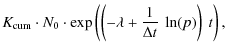
cumulated (the total (integral) number N(t) of all MBPs that have a lifetime of longer than t minutes) number of MBPs (see Fig. 4)
were fitted with an exponential function decreasing with lifetime (for
an interpretation of the fit coefficients see Table 1):
Table 1: Explanation of the different fitting parameters used for Eq. (1).
The exponentially decreasing number of MBPs can be caused by the physics of the process under estimation and/or by the used algorithm. If we take into account that the algorithm has a certain probability p to find an MBP once, then the probability to find the same MBP in the next image again would be p2. For n images we achieve pn which leads to:
where
![\begin{figure}
\par\includegraphics[width=8cm,clip]{13085f04.eps}
\end{figure}](/articles/aa/full_html/2010/03/aa13085-09/img37.png)
|
Figure 4:
Cumulated number of MBPs versus lifetime fitted with an exponential
function (solid line) for data set I. The values of the fit represent
the number of MBPs that have a lifetime greater than or equal to the
corresponding x-axis value
|
| Open with DEXTER | |
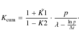
If we suppose that the real number of MBP versus lifetime distribution follows an exponential function,
![]() ,
we find for the measured distribution (for a more elaborate derivation of the measured distribution see the appendix):
,
we find for the measured distribution (for a more elaborate derivation of the measured distribution see the appendix):
| N(t) | = | (4) | |
| = | (5) | ||
| = | 
|
(6) | |
| = | (7) |
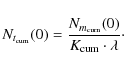
In this context N(t) denotes the measured number of MBPs with a lifetime larger than t. N0 stands for a ``fictitious'' starting number of MBPs. MBPs are formed and decay constantly. If we could force all MBPs to be formed in the first exposure and then could turn off the forming process, N0 would denote the number of features to be found in the first image.
|
(8) |
If we obtain the total decaying constant for data sets with a different temporal sampling
![\begin{figure}
\par\includegraphics[width=8cm,clip]{13085f05.eps}
\end{figure}](/articles/aa/full_html/2010/03/aa13085-09/img44.png)
|
Figure 5: Same as Fig. 4 but derived for a reduced sampling rate (only each third image was used). The corresponding temporal resolution is 96 s. The solid line shows a linear fit for the statistically more robust data. The dotted line shows a linear fit for a second ``unresolved'' distribution (for details see text). |
| Open with DEXTER | |
![\begin{figure}
\par\includegraphics[width=8cm,clip]{13085f06.eps}
\end{figure}](/articles/aa/full_html/2010/03/aa13085-09/img45.png)
|
Figure 6: Cumulated number of MBPs versus time for the two different data sets and different temporal samplings. Fits belonging to data set I are shown by solid lines, data set II by dashed lines. The numbers indicate how many images were skipped to artificially decrease the temporal sampling. |
| Open with DEXTER | |
![\begin{figure}
\par\includegraphics[width=8cm,clip]{13085f07.eps}\vspace*{2mm}
\end{figure}](/articles/aa/full_html/2010/03/aa13085-09/img48.png)
|
Figure 7:
Decaying parameter
|
| Open with DEXTER | |
To test wheter this relationship really holds, we artificially reduced
the temporal sampling of our data sets. For each of these realisations,
we got a distribution similar to Fig. 4.
We artificially decreased data set I by interleaving one or two images
(corresponds to images every 64 and 96 s, respectively) and data
set II by interleaving one, two and three images (corresponds to images
every 22, 33 and 44 s, respectively). Interestingly on thus other
realisations is that a tail is forming out of the measurements cloud of
the long-living MBPs of Fig. 4. This can be seen e.g. in Fig. 5,
which shows the cumulated lifetime for an image cadence of 96 s.
This could represent a second (unresolved) distribution, indicated by
the dashed line. Since we only found about 20 MBPs with lifetimes
longer than 15 min, we did not investigate this tail further. The
resulting exponential fits to the histograms are shown together with
the original ones in Fig. 6. It
can be seen that the slope of the distributions is very similar for
skipping 0 images in data set I to skipping 2 images in data set II,
which relate both to a similar temporal sampling of about 30 s (32
to 33 s; compare also Fig. 7). The obtained fit parameters are listed in Table 2. Decreasing the temporal sampling leads to a flattening of the exponential slope. In Fig. 7 we plot the derived decaying constants
![]() versus the temporal resolution, which follows a straight line. From the linear fit to these curve we derived
versus the temporal resolution, which follows a straight line. From the linear fit to these curve we derived
![]() ,
which corresponds to a mean MBP lifetime of
,
which corresponds to a mean MBP lifetime of
![]() min. The second fit parameter gives us after some transformations the identification probability p of the MBP features in single images. This probability has a value of about 90%.
min. The second fit parameter gives us after some transformations the identification probability p of the MBP features in single images. This probability has a value of about 90%.
Table 2: Overview of the measured lifetimes of MBPs.
4.2 Velocities
![\begin{figure}
\par\includegraphics[width=17cm,clip]{13085f08.eps}\vspace*{3mm}
\end{figure}](/articles/aa/full_html/2010/03/aa13085-09/img72.png)
|
Figure 8:
The top left panel shows the x-component of the velocity of identified single MBPs together with a Gaussian fit for data set I. The fit parameters are: |
| Open with DEXTER | |
The MBP velocity distributions were derived by measuring the movement
of the MBPs brightness barycenter.
The barycenter positions were corrected for the satellite pointing
drift as discussed in Sect. 2. We smoothed the velocities by reducing
the available image cadence. The velocity distributions can be fitted
by Gaussian distributions for the x- and y-velocity components (see Fig. 8), respectively. The effective velocity (
![]() )
was fitted by a Rayleigh distribution (see Fig. 9):
)
was fitted by a Rayleigh distribution (see Fig. 9):
In this notation,
Table 3: Overview of the velocity fit coefficients for the Rayleigh distributions (shown in Figs. 10 and 11) for both data sets.
Figure 10 shows
the velocity distributions and Rayleigh fits for data set I obtained by
different temporal sampling rates. For detailed information about the
fit coefficients derived for different smoothing levels we refer to
Table 3. Figure 11
shows the Rayleigh fits of these distributions all together in one
plot. It can be seen in both figures that the velocity distribution
shows a scaling behaviour with the ![]() -parameter.
As we have only changed the temporal sampling rates, we know that there
has to be some relation between these parameters. We have tried to find
this relation between the
-parameter.
As we have only changed the temporal sampling rates, we know that there
has to be some relation between these parameters. We have tried to find
this relation between the ![]() coefficient of the Rayleigh distribution and the corresponding temporal (
coefficient of the Rayleigh distribution and the corresponding temporal (![]() )
sampling rate. We applied the following empirical relationship:
)
sampling rate. We applied the following empirical relationship:
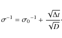
In units of measure D corresponds to a diffusion parameter of an ensemble of MBPs. This means that this parameter should describe the random movement and spreading of a population of MBPs (not to be mixed up with the diffusion of the magnetic field of a single MBP). The application of this relation as a fit function on our data sets is shown in Fig. 12. We obtained the fit parameters
5 Summary and discussion
![\begin{figure}
\par\includegraphics[width=8cm,clip]{13085f09.eps}
\end{figure}](/articles/aa/full_html/2010/03/aa13085-09/img95.png)
|
Figure 9:
Effective velocity
|
| Open with DEXTER | |
Table 4: Overview on MBP lifetimes in earlier studies.
![\begin{figure}
\par\includegraphics[width=15cm,clip]{13085f10.eps}\vspace*{0.2mm}
\end{figure}](/articles/aa/full_html/2010/03/aa13085-09/img100.png)
|
Figure 10:
MBP velocity distribution for different smoothing levels for data set I. The temporal resolution is reduced from the top left panel (each image used;
|
| Open with DEXTER | |
We have further extended the detection and identification algorithm for MBPs described in Utz et al. (2009a).
It consists of an additional processing step, which enables us to
analyse the time series of G-band images. We found MBP velocity and
lifetime distributions in accordance with earlier publications. The
lifetime distribution shows an exponential decrease for longer
lifetimes. The decaying parameter was found to be 0.4
![]() corresponding to a mean lifetime of 2.5 min. We outlined a way to
estimate the identification probability of the algorithm (about 90%)
and to correct the lifetimes for the effects of imperfect detection.
corresponding to a mean lifetime of 2.5 min. We outlined a way to
estimate the identification probability of the algorithm (about 90%)
and to correct the lifetimes for the effects of imperfect detection.
If we compare our lifetime-result with previous studies (see Table 4), we see that lifetimes obtained by automated feature tracking algorithms tend to be shorter than those measured by visual identification and tracking. The reason for this could be that if we identify a feature in a certain exposure visually, we would try to find the same feature in the previous and subsequent images. Since we presume that in the next or previous image the same MBP feature will be found, we tend to identify structures as beginning or decaying MBPs (even when they are too weak to be identified by an automated identification routine or are possiblly unrelated features) that we would not identify if we had no clue about the temporal evolution. The results also depend on how the network and inter-network fields are defined and observed. In de Wijn et al. (2008) small-scale fields were first identified in magnetograms; on the other hand, in de Wijn et al. (2005) MBPs were used as proxies for the magnetic field resulting in a difference of the derived lifetimes of a factor of three.
Our results suggest that the different values for MBP lifetimes are
related to different data sets (sampling) and methods but may also
depend on the amount of magnetic flux in the region of interest, i.e.
depending on the local physical properties of the solar photosphere.
Near large magnetic flux regions such as plages or sunspots, MBP
lifetime could be larger as a result than in quiet Sun regions. This
can be explained if one keeps in mind that the dissipation of large
amounts of flux would in turn also take longer. Our results, obtained
from the analysis of isolated MBPs agree with de Wijn et al. (2005).
In this work, the authors excluded network regions (i.e., MBP chains)
from the analysis through the use of Ca II H maps. The selection of
isolated bright features in both the de Wijn et al. (2005)
analysis and the analysis reported here is the most plausible argument
to explain the agreement above cited. The second unresolved
distribution at larger lifetimes in Fig. 5 may be related to small
patches of active network in our datasets. Although we aimed to exclude
active patches (characterised by grouped MBPs) in our study, it could
happen that some points were still identified (we note that Fig. 5
shows in total only about 20 of these events). The derived effective
velocity distribution was fitted by a Rayleigh distribution. We saw
that the velocity distribution depends on the temporal resolution.
Depending on this sampling effect we estimated the Rayleigh fit
parameter to be in the range of 0.7 to 1.4
![]() .
This corresponds to mean velocities of 0.9 to 1.8
.
This corresponds to mean velocities of 0.9 to 1.8
![]() .
The true
.
The true ![]() -parameter for the Rayleigh velocity distribution was estimated to be 1.6
-parameter for the Rayleigh velocity distribution was estimated to be 1.6
![]() ,
which corresponds to a mean velocity of about 2.0
,
which corresponds to a mean velocity of about 2.0
![]() .
.
To estimate the velocity of the MBPs we used the brightness barycenter to get their positions and subsequently their velocities. Alternatively we could have measured the movement of the brightest pixel of an identified feature. Both methods have their advantages and disadvantages. Measuring the movement by tracking the brightest pixel of a feature is unique and not dependant on the shape of a feature. On the other hand this method leaves only a few possibilities of movement due to the achievable spatial sampling (in principle: up/down, left/right, and diagonal; one or two pixels). Therefore, it would be hard to gain a ``real'' velocity distribution. By taking the method of tracking the barycenter of brightness, many more possibilities are available, as the barycenter coordinates can be determined on sub-pixel resolution. However, this method is sensitive to the morphology of the feature and therefore on the definition of the size of the feature (see also Utz et al. 2009b, on different possibilities of size definition).
Our tracking algorithm estimates the path of a MBP by comparing the
positions of a MBP in two consecutive images. Therefore one is obliged
to choose a certain comparison range, which could be easily estimated
by multiplying the maximum anticipated velocity (about 4
![]() )
by the temporal resolution. If the range is set too small, time series
of MBPs will be broken up, causing the lifetimes and velocities to be
underestimated. On the other hand, by choosing the range to large,
unrelated features will be connected to a time series, which leads to
an overestimation of lifetimes and velocities.
)
by the temporal resolution. If the range is set too small, time series
of MBPs will be broken up, causing the lifetimes and velocities to be
underestimated. On the other hand, by choosing the range to large,
unrelated features will be connected to a time series, which leads to
an overestimation of lifetimes and velocities.
![\begin{figure}
\par\includegraphics[width=8cm,clip]{13085f11.eps} \vspace*{3mm}
\end{figure}](/articles/aa/full_html/2010/03/aa13085-09/img101.png)
|
Figure 11: Comparison of all Rayleigh function fits to the velocity distributions plotted in Fig. 10. The broadness of the distribution as well as the mean velocity of the MBPs decreases with increasing smoothing level (from red to blue), i.e. lower time cadence. |
| Open with DEXTER | |
To get a real velocity distribution rather than just a few velocity ``states''![]() we have to smooth our obtained velocity values. The smoothing of the
distributions has several effects. First of all the distribution gets
``closer'' to the real distribution as there are now more possible
velocity states. On the other hand the measured velocity decreases and
the distribution gets narrower. This can be explained by the movement
of a feature on the solar disc. This movement consists of two parts, a
deterministic movement and a chaotic movement component. The
deterministic movement is due to large scale flows, e.g., supergranular
flows, meridional circulation etc. These can cause MBPs to move over
larger spatial scales and longer time scales with preferred directions
and velocities than just moving randomly. The chaotic movement is due
to random processes and corresponds to a ``zigzag'' path of a feature
on the solar disc
(for implications of this random walk on the diffusive magnetic field
transport see e.g. Berger et al. 1998; Stanislavsky & Weron 2009,2007).
This yields a dependence of the length of the path on the temporal
resolution of the observations. Consequently the shorter the temporal
lags between the observations, the more accurate is the measurement of
the path and the longer the path will be (one could observe more zigzag
steps).
So we have learned that by smoothing (artificially decreasing the time
cadence), the derived MBP velocity decreases. This is not only true for
MBP movements but holds also for other motions, as can be seen e.g. Attie et al. (2009)
who investigated granular flow field maps and found a similar
behaviour. On the other hand, if we do not smooth, we probably get
velocities which are too high. This is due to the effect that the
temporal to spatial sampling has to have a certain ratio. If we have a
temporal sampling which is too high with respect to the spatial
sampling (for a given velocity), the MBP would stand still for several
exposures. If the feature finally moves, it jumps from one pixel to
another and the derived velocity will be too high, since in reality the
feature moves more or less continuously all the time. On the other
hand, if the time resolution is too low (smoothing too high), we would
loose much of the chaotic movement and derive a ``mean'' velocity which
is too low. Figure 10
shows this effect. We see that in the first cases the distribution is
broader with a high velocity tail. The last two plots show that the
obtained measurement points now concentrate more or less at average
velocities (the distribution gets significantly narrower) and only a
small number of high velocities can be found.
we have to smooth our obtained velocity values. The smoothing of the
distributions has several effects. First of all the distribution gets
``closer'' to the real distribution as there are now more possible
velocity states. On the other hand the measured velocity decreases and
the distribution gets narrower. This can be explained by the movement
of a feature on the solar disc. This movement consists of two parts, a
deterministic movement and a chaotic movement component. The
deterministic movement is due to large scale flows, e.g., supergranular
flows, meridional circulation etc. These can cause MBPs to move over
larger spatial scales and longer time scales with preferred directions
and velocities than just moving randomly. The chaotic movement is due
to random processes and corresponds to a ``zigzag'' path of a feature
on the solar disc
(for implications of this random walk on the diffusive magnetic field
transport see e.g. Berger et al. 1998; Stanislavsky & Weron 2009,2007).
This yields a dependence of the length of the path on the temporal
resolution of the observations. Consequently the shorter the temporal
lags between the observations, the more accurate is the measurement of
the path and the longer the path will be (one could observe more zigzag
steps).
So we have learned that by smoothing (artificially decreasing the time
cadence), the derived MBP velocity decreases. This is not only true for
MBP movements but holds also for other motions, as can be seen e.g. Attie et al. (2009)
who investigated granular flow field maps and found a similar
behaviour. On the other hand, if we do not smooth, we probably get
velocities which are too high. This is due to the effect that the
temporal to spatial sampling has to have a certain ratio. If we have a
temporal sampling which is too high with respect to the spatial
sampling (for a given velocity), the MBP would stand still for several
exposures. If the feature finally moves, it jumps from one pixel to
another and the derived velocity will be too high, since in reality the
feature moves more or less continuously all the time. On the other
hand, if the time resolution is too low (smoothing too high), we would
loose much of the chaotic movement and derive a ``mean'' velocity which
is too low. Figure 10
shows this effect. We see that in the first cases the distribution is
broader with a high velocity tail. The last two plots show that the
obtained measurement points now concentrate more or less at average
velocities (the distribution gets significantly narrower) and only a
small number of high velocities can be found.
Another interesting aspect is that not only the shape of the distribution but also the mean value of the distribution is changed. This is due to the fact that we have a non-symmetric function. In the process of smoothing, more of the high values are redistributed to lower values than vice versa. This is the mathematical explanation. The technical interpretation is that we loose a part of the MBPs path by reducing the temporal sampling. This leads to the shift of the distribution which can be seen in Fig. 11.
![\begin{figure}
\par\includegraphics[width=8cm,clip]{13085f12.eps}
\vspace*{3mm}
\end{figure}](/articles/aa/full_html/2010/03/aa13085-09/img102.png)
|
Figure 12:
The measured Rayleigh |
| Open with DEXTER | |
![\begin{figure}
\par\includegraphics[width=8cm,clip]{13085f13.eps} \vspace*{3.8mm}
\end{figure}](/articles/aa/full_html/2010/03/aa13085-09/img103.png)
|
Figure 13:
The obtained Rayleigh distribution for the estimated true |
| Open with DEXTER | |
6 Conclusion
In this study we found MBP lifetimes (corrected mean value
![]() min) and velocities (corrected Rayleigh fit parameter
min) and velocities (corrected Rayleigh fit parameter
![]()
![]() )
in the range of earlier reported values. Additionally we investigated
the relationship between image cadence and obtained lifetimes and
velocities. Using the derived relations we were able for the first time
to correct the measured velocity distribution for this influence. The
corrected velocity distribution shows many more fast moving MBPs (
)
in the range of earlier reported values. Additionally we investigated
the relationship between image cadence and obtained lifetimes and
velocities. Using the derived relations we were able for the first time
to correct the measured velocity distribution for this influence. The
corrected velocity distribution shows many more fast moving MBPs (
![]() )
than the original measured distribution (12% for the corrected
distribution; 0.2% for the measured distribution with the highest
)
than the original measured distribution (12% for the corrected
distribution; 0.2% for the measured distribution with the highest ![]() ;
see also Fig. 13).
The obtained fraction of fast moving MBPs could play a crucial role in
AC coronal heating models. In fact, fast moving MBPs have a large
impact on the amount of energy available for AC heating processes. This
was outlined in the theoretical work of Choudhuri et al. (1993); here the authors individuated in ``fast motions'' (
;
see also Fig. 13).
The obtained fraction of fast moving MBPs could play a crucial role in
AC coronal heating models. In fact, fast moving MBPs have a large
impact on the amount of energy available for AC heating processes. This
was outlined in the theoretical work of Choudhuri et al. (1993); here the authors individuated in ``fast motions'' (![]()
![]() )
of magnetic footpoints a potential source of energy to support the coronal heating.
)
of magnetic footpoints a potential source of energy to support the coronal heating.
We are grateful to the Hinode team for the possibility to use their data. Hinode is a Japanese mission developed and launched by ISAS/JAXA, collaborating with NAOJ as a domestic partner, NASA and STFC (UK) as international partners. Scientific operation of the Hinode mission is conducted by the Hinode science team organized at ISAS/JAXA. This team mainly consists of scientists from institutes in the partner countries. Support for the post-launch operation is provided by JAXA and NAOJ (Japan), STFC (UK), NASA (USA), ESA, and NSC (Norway). This work was supported by FWF Fonds zur Förderung wissenschaftlicher Forschung grant P17024. D.U. and A.H. are grateful to the ÖAD Österreichischer Austauschdienst for financing research visits at the Pic du Midi Observatory. M.R. is grateful to the Ministère des Affaires Étrangères et Européennes, for financing a research visit at the University of Graz. This work was partly supported by the Slovak Research and Development Agency SRDA project APVV-0066-06 (J.R.). We are grateful to the anonymous referee for her/his very detailed remarks and comments, which helped us to present the outcome of this work in a clearer way.
Appendix A: Correction factors for the lifetime distribution
Table A.1:
shows the probability relations (fractional relation) between the true distribution (Nt; indicated by the first row) and the actually measured distribution (![]() ;
indicated by the first column)
;
indicated by the first column)
![]() .
.
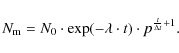
We are now deriving the higher order correction factors for the measured distribution. In Table A.1 we see that there are a lot more elements. The first row (true) indicates the number of MBPs at a certain time instance t. The first column (measured) indicates the measured number of MBPs for a certain time instance t. Every element of a crossing of a row (refering to a certain measured lifetime
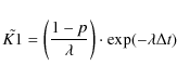
where K1 is:
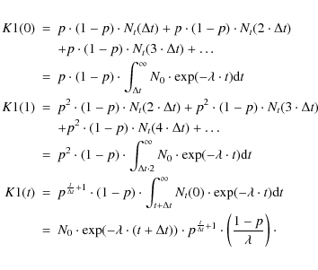
We see that this equation is very similar to Eq. (A.1). Thus we can rewrite Eq. (A.2) as
| Nm | = | (A.3) | |
| Nm | = | (A.4) |
where
|
(A.5) |
is always positive. This value describes the overestimation of the measurement bins of a distribution by erroneously measuring long living features in the short living bins (by loosing track of a feature). Interestingly this factor is time-independent and a constant for certain parameters (detection probability p, time cadence
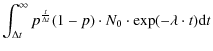
Now we can derive a second order correction parameter. Loosing track of the MBPs does not only lead to erroneously measured MBP lifetimes but also creates a second order lifetime distribution. This can be explained that by loosing track of the MBP, the MBP itself will not disappear. Therefore, it can happen that we will measure the same MBP again in the future. We will now try to estimate a parameter describing this circumstance.
If we move from the principle diagonal in Table A.1
to the next diagonal, this diagonal would describe the probability to
have an MBP in the data set that will live for one time step more than
originally measured. The sum over these elements will give us all
elements that live one more time step. The next diagonal describes the
MBPs that live two more time steps and so on. Therefore, the diagonal
elements describe the truncated part of the original distribution which
forms itself a new distribution. We will derive this distribution now:
| |
= | ||
| (A.6) | |||
| = | 
|
(A.7) | |
| = | (A.8) | ||
| = | 
|
(A.9) | |
| = | 
|
(A.10) | |
| = | 
|
(A.11) | |
| = | 
|
(A.12) | |
| = | (A.13) |
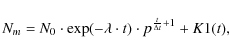
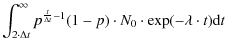
where K2 is given by:
|
(A.14) |
This factor K2 describes the creation of the new distribution (the truncated one), which also contributes to the measured distribution. This truncated distribution gives rise to a truncated-truncated distribution and so forth. Finally, we arrive at the following measured distribution:
| |
= | ||
| (A.15) | |||
| = | 
|
(A.16) | |
| = | 
|
(A.17) |
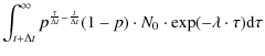
As a last point, we want to give the equation for the cumulated number-lifetime measurement distribution of the MBPs:
| |
= | 
|
(A.18) |
| = | 
|
||
|
(A.19) | ||
| = | 
|
(A.20) |
where
|
(A.21) |
If we compare this with the true cumulated distribution
|
(A.22) |
References
- Attie, R., Innes, D. E., & Potts, H. E. 2009, A&A, 493, L13
- Beck, C., Bellot Rubio, L. R., Schlichenmaier, R., & Sütterlin, P. 2007, A&A, 472, 607
- Berger, T. E., & Title, A. M. 1996, ApJ, 463, 365
- Berger, T. E., & Title, A. M. 2001, ApJ, 553, 449
- Berger, T. E., Löfdahl, M. G., Shine, R. A., & Title, A. M. 1998, ApJ, 506, 439
- Berger, T. E., Rouppe van der Voort, L. H. M., Löfdahl, M. G., et al. 2004, A&A, 428, 613
- Bharti, L., Jain, R., Joshi, C., & Jaaffrey, S. N. A. 2006, in ASP Conf. Ser. 358, ed. R. Casini, & B. W. Lites, 61
- Choudhuri, A. R., Auffret, H., & Priest, E. R. 1993, Sol. Phys., 143, 49
- de Wijn, A. G., Rutten, R. J., Haverkamp, E. M. W. P., & Sütterlin, P. 2005, A&A, 441, 1183
- de Wijn, A. G., Lites, B. W., Berger, T. E., et al. 2008, ApJ, 684, 1469
- Deinzer, W., Hensler, G., Schuessler, M., & Weisshaar, E. 1984a, A&A, 139, 426
- Deinzer, W., Hensler, G., Schussler, M., & Weisshaar, E. 1984b, A&A, 139, 435
- Hasan, S. S., van Ballegooijen, A. A., Kalkofen, W., & Steiner, O. 2005, ApJ, 631, 1270
- Ichimoto, K., Tsuneta, S., Suematsu, Y., et al. 2004, in Optical, Infrared, and Millimeter Space Telescopes, Presented at the Society of Photo-Optical Instrumentation Engineers (SPIE) Conference, ed. J. C. Mather, Proc. SPIE, 5487, 1142
- Ichimoto, K., Katsukawa, Y., Tarbell, T., et al. 2008, in First Results From Hinode, ed. S. A. Matthews, J. M. Davis, & L. K. Harra, ASP Conf. Ser., 397, 5
- Keller, C. U. 1992, Nature, 359, 307
- Kosugi, T., Matsuzaki, K., Sakao, T., et al. 2007, Sol. Phys., 243, 3
- Möstl, C., Hanslmeier, A., Sobotka, M., Puschmann, K., & Muthsam, H. J. 2006, Sol. Phys., 237, 13
- Muller, R. 1983, Sol. Phys., 85, 113
- Muller, R., & Keil, S. L. 1983, Sol. Phys., 87, 243
- Muller, R., & Roudier, T. 1992, Sol. Phys., 141, 27
- Muller, R., Roudier, T., Vigneau, J., & Auffret, H. 1994, A&A, 283, 232
- Osherovich, V. A., Chapman, G. A., & Fla, T. 1983, ApJ, 268, 412
- Parker, E. N. 1983, ApJ, 264, 642
- Parker, E. N. 1988, ApJ, 330, 474
- Rutten, R. J. 1999, in Third Advances in Solar Physics Euroconference: Magnetic Fields and Oscillations, ed. B. Schmieder, A. Hofmann, & J. Staude, ASP Conf. Ser., 184, 181
- Sánchez Almeida, J., Márquez, I., Bonet, J. A., Domínguez Cerdeña, I., & Muller, R. 2004, ApJ, 609, L91
- Schüssler, M., Shelyag, S., Berdyugina, S., Vögler, A., & Solanki, S. K. 2003, ApJ, 597, L173
- Shelyag, S., Erdélyi, R., & Thompson, M. J. 2006, ApJ, 651, 576
- Spruit, H. C. 1976, Sol. Phys., 50, 269
- Stanislavsky, A., & Weron, K. 2009, Ap&SS, 104
- Stanislavsky, A. A., & Weron, K. 2007, Ap&SS, 312, 343
- Steiner, O., Grossmann-Doerth, U., Knoelker, M., & Schuessler, M. 1998, ApJ, 495, 468
- Steiner, O., Hauschildt, P. H., & Bruls, J. 2001, A&A, 372, L13
- Suematsu, Y., Tsuneta, S., Ichimoto, K., et al. 2008, Sol. Phys., 26
- Utz, D., Hanslmeier, A., Möstl, C., et al. 2009a, A&A, 498, 289
- Utz, D., Hanslmeier, A., Muller, R., et al. 2009b, Central European Astrophysical Bulletin, 33, 29
- Viticchié, B., Del Moro, D., Berrilli, F., Bellot Rubio, L., & Tritschler, A. 2009, ApJ, 700, L145
- Vögler, A., Shelyag, S., Schüssler, M., et al. 2005, A&A, 429, 335
- Wiehr, E., Bovelet, B., & Hirzberger, J. 2004, A&A, 422, L63
- Yi, Z., & Engvold, O. 1993, Sol. Phys., 144, 1
Footnotes
- ... ``states''
![[*]](/icons/foot_motif.png)
- A state is a possible velocity value. As we are working with discretised data, there are no arbritrary displacement possibilities and therefore also the velocity values are not arbritary. Some velocity values are a lot more favourable (no movement, one pixel in a direction, ...) than others. Calculating displacements by barycenters instead of calculating them by the difference of the brightest pixel helps, but as the sizes are very small the displacement states mentioned before are still more favourable.
- ...
- As an example, let us think of the real number of MBPs at
time instance 2
 Nt(2)),
this number is measured (contributes) by a factor of p3
reduced for the measured Nm(2). But not
only the true
number of MBPs at a certain lifetime contribute to the measured value
of this lifetime. If we consider the measured number of MBPs at
time ,
we see that the true number of MBPs at time 3. contributes with a fraction
of p2(1-p) to the measured number of
MBPs at a lifetime
of .
To get a correct distribution all of these relations have to be
considered (see text).
Nt(2)),
this number is measured (contributes) by a factor of p3
reduced for the measured Nm(2). But not
only the true
number of MBPs at a certain lifetime contribute to the measured value
of this lifetime. If we consider the measured number of MBPs at
time ,
we see that the true number of MBPs at time 3. contributes with a fraction
of p2(1-p) to the measured number of
MBPs at a lifetime
of .
To get a correct distribution all of these relations have to be
considered (see text).
All Tables
Table 1: Explanation of the different fitting parameters used for Eq. (1).
Table 2: Overview of the measured lifetimes of MBPs.
Table 3: Overview of the velocity fit coefficients for the Rayleigh distributions (shown in Figs. 10 and 11) for both data sets.
Table 4: Overview on MBP lifetimes in earlier studies.
Table A.1:
shows the probability relations (fractional relation) between the true distribution (Nt; indicated by the first row) and the actually measured distribution (![]() ;
indicated by the first column)
;
indicated by the first column)
![]() .
.
All Figures
|
|
Figure 1:
Hinode/SOT pointing stability for data sets I ( left) and II ( right). Top row: the displacement between an image and the succeeding one ( |
| Open with DEXTER | |
| In the text | |
|
|
Figure 2: Top panel: starting frame of one of the identified MBPs. Bottom panels: evolution (time series) of the detected MBP in the rectangle. The white cross marks the derived brightness barycenter. The path of the MBP is shown as a white line. Positions are given in arcsec from the bottom left corner of the full frame. |
| Open with DEXTER | |
| In the text | |
|
|
Figure 3: Histogram of the obtained MBP lifetimes of data set I together with an exponential fit (solid line). The histogram was normalised by dividing the counts in each bin by the binsize. The histogram is only shown up to the first zero crossing, i.e. there are a few longer-living MBPs than shown in the figure. |
| Open with DEXTER | |
| In the text | |
|
|
Figure 4:
Cumulated number of MBPs versus lifetime fitted with an exponential
function (solid line) for data set I. The values of the fit represent
the number of MBPs that have a lifetime greater than or equal to the
corresponding x-axis value
|
| Open with DEXTER | |
| In the text | |
|
|
Figure 5: Same as Fig. 4 but derived for a reduced sampling rate (only each third image was used). The corresponding temporal resolution is 96 s. The solid line shows a linear fit for the statistically more robust data. The dotted line shows a linear fit for a second ``unresolved'' distribution (for details see text). |
| Open with DEXTER | |
| In the text | |
|
|
Figure 6: Cumulated number of MBPs versus time for the two different data sets and different temporal samplings. Fits belonging to data set I are shown by solid lines, data set II by dashed lines. The numbers indicate how many images were skipped to artificially decrease the temporal sampling. |
| Open with DEXTER | |
| In the text | |
|
|
Figure 7:
Decaying parameter
|
| Open with DEXTER | |
| In the text | |
|
|
Figure 8:
The top left panel shows the x-component of the velocity of identified single MBPs together with a Gaussian fit for data set I. The fit parameters are: |
| Open with DEXTER | |
| In the text | |
|
|
Figure 9:
Effective velocity
|
| Open with DEXTER | |
| In the text | |
|
|
Figure 10:
MBP velocity distribution for different smoothing levels for data set I. The temporal resolution is reduced from the top left panel (each image used;
|
| Open with DEXTER | |
| In the text | |
|
|
Figure 11: Comparison of all Rayleigh function fits to the velocity distributions plotted in Fig. 10. The broadness of the distribution as well as the mean velocity of the MBPs decreases with increasing smoothing level (from red to blue), i.e. lower time cadence. |
| Open with DEXTER | |
| In the text | |
|
|
Figure 12:
The measured Rayleigh |
| Open with DEXTER | |
| In the text | |
|
|
Figure 13:
The obtained Rayleigh distribution for the estimated true |
| Open with DEXTER | |
| In the text | |
Copyright ESO 2010
Current usage metrics show cumulative count of Article Views (full-text article views including HTML views, PDF and ePub downloads, according to the available data) and Abstracts Views on Vision4Press platform.
Data correspond to usage on the plateform after 2015. The current usage metrics is available 48-96 hours after online publication and is updated daily on week days.
Initial download of the metrics may take a while.