| Issue |
A&A
Volume 509, January 2010
|
|
|---|---|---|
| Article Number | A54 | |
| Number of page(s) | 18 | |
| Section | Extragalactic astronomy | |
| DOI | https://doi.org/10.1051/0004-6361/200912903 | |
| Published online | 19 January 2010 | |
Radio counterpart of the lensed submm emission in the cluster MS0451.6-0305: new evidence for the merger scenario
A. Berciano Alba1,2 - L. V. E. Koopmans2 - M. A. Garrett1,3,4 - O. Wucknitz5 - M. Limousin6,7
1 - Netherlands Foundation for Research in Astronomy (ASTRON),
Postbus 2, 7990 AA Dwingeloo, The Netherlands
2 - Kapteyn
Astronomical Institute, University of Groningen, PO Box 800, 9700
AV, Groningen, The Netherlands
3 - Leiden Observatory, PO Box 9513,
2300 RA, Leiden, The Netherlands
4 - Centre for Astrophysics and
Supercomputing, Swinburne University of Technology, Mail number H39,
PO Box 218, Hawthorn, Victoria 3122, Australia
5 - Argelander-Institut für Astronomie (AIfA), University of Bonn, Auf
dem Hügel 71, 53121 Bonn, Germany
6 - Laboratoire d'Astrophysique
de Marseille, UMR 6110, CNRS-Université de Provence, 38 rue
Frédéric Joliot-Curie, 13 388 Marseille Cedex 13, France
7 - Dark Cosmology Centre, Niels Bohr Institute, University of
Copenhagen,
Juliane Maries Vej 30, 2100 Copenhagen, Denmark
Received 16 July 2009 / Accepted 7 September 2009
Abstract
Context. SMM J04542-0301 is an extended (![]()
![]() )
submm source located near the core of the cluster MS0451.6-0305. It has
been suggested that part of its emission arises from the interaction
between a LBG and two EROs at
)
submm source located near the core of the cluster MS0451.6-0305. It has
been suggested that part of its emission arises from the interaction
between a LBG and two EROs at ![]() that are multiply-imaged in the optical/NIR observations. However, the
dramatic resolution difference between the sub-mm map and the
optical/NIR images make it difficult to confirm this hypothesis.
that are multiply-imaged in the optical/NIR observations. However, the
dramatic resolution difference between the sub-mm map and the
optical/NIR images make it difficult to confirm this hypothesis.
Aims. In a previous paper, we reported the detection
of 1.4 GHz continuum radio emission coincident with this
sub-mm source using VLA archival data. To fully understand the relation
between this radio emission, the sub-mm emission, and the optical/IR
multiply-imaged sources, we have re-observed the cluster with the VLA
at higher resolution.
Methods. The previous archival data has been
re-reduced and combined with the new observations to produced a deep (![]() 10
10 ![]() Jy beam-1),
high resolution (
Jy beam-1),
high resolution (![]()
![]() )
map centred on the cluster core. The strong lensing effect in the radio
data has been quantified by constructing a new lens model of the
cluster.
)
map centred on the cluster core. The strong lensing effect in the radio
data has been quantified by constructing a new lens model of the
cluster.
Results. From the high resolution map we have
robustly identified six radio sources located within
SMM J 04542-0301. The brightest and most extended of
these sources (RJ) is located in the middle of the sub-mm emission, and
has no obvious counterpart in the optical/NIR. Three other detections
(E1, E2 and E3) seem to be associated with the images of one of the
EROs (B), although the NIR and radio emission appear to originate at
slightly different positions in the source plane. The last two
detections (CR1 and CR2), for which no optical/NIR counterpart have
been found, seem to constitute two relatively compact emitting regions
embedded in a ![]()
![]() extended
radio source located at the position of the sub-mm peak. The presence
of this extended component (which contributes 38% of the total radio
flux in this region) can only be explained if it is being produced by a
lensed region of dust obscured star formation in the center of the
merger. A comparison between the radio and sub-mm data at the same
resolution suggests that E1, E2, E3, CR1 and CR2 are associated with
the sub-mm emission.
extended
radio source located at the position of the sub-mm peak. The presence
of this extended component (which contributes 38% of the total radio
flux in this region) can only be explained if it is being produced by a
lensed region of dust obscured star formation in the center of the
merger. A comparison between the radio and sub-mm data at the same
resolution suggests that E1, E2, E3, CR1 and CR2 are associated with
the sub-mm emission.
Conclusions. The radio observations presented in
this paper provide strong observational evidence in favour of the
merger hypothesis. However, the question if RJ is also contributing to
the observed sub-mm emission remains open. These results illustrate the
promising prospects for radio interferometry and strong gravitational
lensing to study the internal structure of SMGs.
Key words: galaxies: clusters: individual: SMM J 04542-0301 - galaxies: starburst - radio continuum: galaxies - galaxies: interactions - gravitational lensing: strong
1 Introduction
The detection of the cosmic infrared background (CIB) by the COBE
satellite (Puget
et al. 1996; Hauser et al. 1998)
established that about half of the
total radiation in the universe comes from dust-obscured galaxies that
are missing from optical surveys (see Lagache
et al. 2005, for a
review). This population of dusty objects was first
resolved by the IRAS and ISO satellites up to ![]() ,
and turned out
to be dominated by luminous and ultra-luminous IR galaxies (LIRGs and
ULIRGs). The step into the high-z universe came with
the advent of
sub-mm and mm surveys, since the far-infrared (FIR) luminosity peak of
high-z obscured galaxies is red-shifted into the
sub-mm band
(Blain
& Longair 1993; Franceschini et al. 1991).
As a result, sub-mm galaxies
(hereafter SMGs) turned out to be hundreds of times more numerous than
galaxies with similar luminosities in the local universe, suggesting
that they constitute the dominant contributor of the CIB and cosmic
star formation at
,
and turned out
to be dominated by luminous and ultra-luminous IR galaxies (LIRGs and
ULIRGs). The step into the high-z universe came with
the advent of
sub-mm and mm surveys, since the far-infrared (FIR) luminosity peak of
high-z obscured galaxies is red-shifted into the
sub-mm band
(Blain
& Longair 1993; Franceschini et al. 1991).
As a result, sub-mm galaxies
(hereafter SMGs) turned out to be hundreds of times more numerous than
galaxies with similar luminosities in the local universe, suggesting
that they constitute the dominant contributor of the CIB and cosmic
star formation at ![]() .
This illustrates the very important
role that SMGs play in the context of galaxy formation and evolution
(see Lonsdale et al. 2006,
for a review on (U)LIRGs and SMGs).
.
This illustrates the very important
role that SMGs play in the context of galaxy formation and evolution
(see Lonsdale et al. 2006,
for a review on (U)LIRGs and SMGs).
One decade after their discovery with SCUBA![]() (Smail
et al. 1997; Barger et al. 1998; Eales
et al. 1999; Hughes et al. 1998), it is
generaly acepted
that SMGs are heavily dust-obscured galaxies at high redshift (2<z
<3) with ULIRG-like luminosities (
(Smail
et al. 1997; Barger et al. 1998; Eales
et al. 1999; Hughes et al. 1998), it is
generaly acepted
that SMGs are heavily dust-obscured galaxies at high redshift (2<z
<3) with ULIRG-like luminosities (
![]() )
and star formation rates of the order of 1000
)
and star formation rates of the order of 1000 ![]() yr-1.
This enormous bolometric luminosity seems to be
dominated by star formation processes induced by galaxy
interactions/mergers, although a good fraction (
yr-1.
This enormous bolometric luminosity seems to be
dominated by star formation processes induced by galaxy
interactions/mergers, although a good fraction (![]()
![]() )
of
SMGs also host AGN activity (Alexander
et al. 2005). First estimates of their
physical properties indicate that SMGs are massive, gas rich systems
(
)
of
SMGs also host AGN activity (Alexander
et al. 2005). First estimates of their
physical properties indicate that SMGs are massive, gas rich systems
(
![]() )
in which the starburst
region has a typical scale in the range 1-8 kpc (Biggs &
Ivison 2008; Chapman
et al. 2004; Greve et al. 2005; Wang et al.
2007; Tacconi
et al. 2006; Neri et al. 2003). The
available evidence also
suggests that SMGs might be the progenitors of massive local
ellipticals (Webb
et al. 2003; Smail et al. 2004; Alexander
et al. 2003; Genzel et al. 2003; Alexander
et al. 2005; Smail et al. 2002; Lilly
et al. 1999; Swinbank et al. 2006).
)
in which the starburst
region has a typical scale in the range 1-8 kpc (Biggs &
Ivison 2008; Chapman
et al. 2004; Greve et al. 2005; Wang et al.
2007; Tacconi
et al. 2006; Neri et al. 2003). The
available evidence also
suggests that SMGs might be the progenitors of massive local
ellipticals (Webb
et al. 2003; Smail et al. 2004; Alexander
et al. 2003; Genzel et al. 2003; Alexander
et al. 2005; Smail et al. 2002; Lilly
et al. 1999; Swinbank et al. 2006).
However, these general properties of SMGs are based on the
study of
the very brightest examples of this class of object (
![]() mJy),
and may not be representative of the entire SMG
population. In fact, according to Knudsen
et al. (2008), the dominant
contribution to the sub-mm extragalactic background comes from the
fainter (sub-)mJy sources that cannot usually be detected due to the
confusion noise of current instruments (
mJy),
and may not be representative of the entire SMG
population. In fact, according to Knudsen
et al. (2008), the dominant
contribution to the sub-mm extragalactic background comes from the
fainter (sub-)mJy sources that cannot usually be detected due to the
confusion noise of current instruments (
![]() mJy).
The only way in which it has been possible to push bellow
this sensitivity limit, is by using the lensing magnification provided
by massive clusters of galaxies to increase the effective resolution
of SCUBA. This approach has improved the sensitivity of sub-mm maps by
factors of a few with respect to blank field surveys, although just a
handfull of faint SMGs have being identified so far (Cowie
et al. 2002; Knudsen et al. 2008; Smail
et al. 2002). Since so little is known about these
intrinsically
faint sources, it is crucial to further investigate their properties
(e.g. spectral energy distributions, morphologies, redshifts, etc.)
and assess whether they are different from the observed properties of
brighter SMGs.
mJy).
The only way in which it has been possible to push bellow
this sensitivity limit, is by using the lensing magnification provided
by massive clusters of galaxies to increase the effective resolution
of SCUBA. This approach has improved the sensitivity of sub-mm maps by
factors of a few with respect to blank field surveys, although just a
handfull of faint SMGs have being identified so far (Cowie
et al. 2002; Knudsen et al. 2008; Smail
et al. 2002). Since so little is known about these
intrinsically
faint sources, it is crucial to further investigate their properties
(e.g. spectral energy distributions, morphologies, redshifts, etc.)
and assess whether they are different from the observed properties of
brighter SMGs.
A promissing strategy to gather information about faint SMGs is to study members that are multiply imaged by clusters of galaxies. In this cases, the magnification factor can go up to 30 (or more), providing not only the opportunity to detect but also to spatially resolve the morphologies and internal dynamics of faint SMGs at a level of detail far greater than would otherwise be possible (see Swinbank et al. 2007, for an example of this technique in the optical). To date, only one multiply-imaged faint SMGs has been confirmed: SMM J16359+6612, located near the core of the cluster A2218 (Knudsen et al. 2009,2008; Garrett et al. 2005; Kneib et al. 2005,2004). There are, however, two other clusters which seem to host multiply-imaged SMGs: A1689 (Knudsen et al. 2008) and MS0451.6-0305 (Chapman et al. 2002; Berciano Alba et al. 2007; Borys et al. 2004).
![\begin{figure}
\par\includegraphics[width=8.5cm,clip]{12903fg1.ps}
\end{figure}](/articles/aa/full_html/2010/01/aa12903-09/img44.png)
|
Figure 1:
Summary of the results presented in
Borys et al. (2004).
SCUBA |
| Open with DEXTER | |
The case of MS0451.6-0305 is particularly interesting, since the
``sub-mm source'' (SMM J04542-0301) is an elongated (![]()
![]() )
region of
)
region of ![]() m
emission which is coincident with an
optical arc and five NIR sources (see Fig. 1). While the
optical arc is the result of a strongly-lensed Lyman Break Galaxy
(LBG) at
m
emission which is coincident with an
optical arc and five NIR sources (see Fig. 1). While the
optical arc is the result of a strongly-lensed Lyman Break Galaxy
(LBG) at ![]() ,
a lens model of the cluster predicts
that the set of NIR sources could be produced by two triply-imaged
EROs
,
a lens model of the cluster predicts
that the set of NIR sources could be produced by two triply-imaged
EROs![]() located at almost the same
redshift (
located at almost the same
redshift (
![]() ).
The model also indicates that the ERO pair and the LBG may
constitute a merger at z=2.9 in the source plane,
with their
interaction likely being at the origin of the observed sub-mm emission
(Borys et al. 2004,
B04 hereafter). Unfortunately, the low resolution
(
).
The model also indicates that the ERO pair and the LBG may
constitute a merger at z=2.9 in the source plane,
with their
interaction likely being at the origin of the observed sub-mm emission
(Borys et al. 2004,
B04 hereafter). Unfortunately, the low resolution
(![]()
![]() at
at ![]() m) and poor
positional accuracy (
m) and poor
positional accuracy (![]()
![]() rms)
of SCUBA, makes it very difficult to confirm
the link between SMM J04542-0301 and the proposed optical/NIR
sources. Moreover, the emission coming from the north-eastern and
central regions of the sub-mm emission cannot be reproduced by the arc
and the NIR sources (see Fig. 7 in B04), suggesting that it
might
arise via other sources.
rms)
of SCUBA, makes it very difficult to confirm
the link between SMM J04542-0301 and the proposed optical/NIR
sources. Moreover, the emission coming from the north-eastern and
central regions of the sub-mm emission cannot be reproduced by the arc
and the NIR sources (see Fig. 7 in B04), suggesting that it
might
arise via other sources.
A possible way to overcome this resolution problem is by
taking
advantage of the observed correlation between the radio synchrotron
and FIR emission in star-forming galaxies
(Garrett 2002;
Beelen
et al. 2006; van der Kruit 1971;
Helou
et al. 1985; Appleton et al. 2004; Condon
et al. 1982), which also seems to
hold for SMGs out to ![]() (Vlahakis
et al. 2007; Kovács et al. 2006; Michaowski
et al. 2009; Ibar et al. 2008). Thanks
to this FIR-radio
correlation, radio interferometric observations can be used as a
high-resolution proxy for the rest-frame FIR emission observed in the
sub-mm. This approach has been extensively used to pinpoint the
position of SMGs in order to identify their faint optical counterparts
(e.g. Ivison
et al. 2000,2007; Barger et al. 2000; Chapman
et al. 2005).
(Vlahakis
et al. 2007; Kovács et al. 2006; Michaowski
et al. 2009; Ibar et al. 2008). Thanks
to this FIR-radio
correlation, radio interferometric observations can be used as a
high-resolution proxy for the rest-frame FIR emission observed in the
sub-mm. This approach has been extensively used to pinpoint the
position of SMGs in order to identify their faint optical counterparts
(e.g. Ivison
et al. 2000,2007; Barger et al. 2000; Chapman
et al. 2005).
In Berciano Alba
et al. (2007), we reported the detection
of 1.4 GHz radio emission
coincident with SMM J04542-0301 using VLA![]() archival data. Part of this radio emission is located in the region
between the optical arc and the ERO images, which is consistent with
the interacting region of the hypothetical merger being the source of
the observed radio and sub-mm emission. We also detected bright radio
emission in the central region of SMM J04542-0301, although it
is
not clear if this emission is produced by a high-z
lensed object or
AGN activity associated with a cluster member.
archival data. Part of this radio emission is located in the region
between the optical arc and the ERO images, which is consistent with
the interacting region of the hypothetical merger being the source of
the observed radio and sub-mm emission. We also detected bright radio
emission in the central region of SMM J04542-0301, although it
is
not clear if this emission is produced by a high-z
lensed object or
AGN activity associated with a cluster member.
In this paper, we present a higher resolution 1.4 GHz radio map of the center of the cluster MS0451.6-0305 (MS0451 hereafter), obtained after combining the previous VLA archival data (BnA configuration) with new VLA high resolution observations (A configuration). The details of both sets of observations are presented in Sect. 2, together with a description of the data analysis procedure, which has been considerably improved with respect to Berciano Alba et al. (2007). Section 3 is dedicated to the analysis of the final combined data set, from which we characterise the compact and extended radio emission detected within SMM J04542-0301. Identification of optical (HST/ACS F814W) and NIR (SUBARU/CISCO K' band) counterparts for the radio detections, as well as their connection with the sub-mm emission, is discussed in Sect. 4. In Sect. 5 we describe a new lens model of the cluster MS0451.6-0305, built to investigate the lensed nature of the compact radio detections. A discussion about the merger scenario proposed by Borys et al. (2004) including the results from the radio observations are presented in Sect. 6. Summary and conclusions are presented in Sect. 7.
The adopted cosmology corresponds to a ![]() CDM model with
CDM model with
![]() ,
,
![]() and h0=73(Spergel et al. 2007).
and h0=73(Spergel et al. 2007).
2 Radio observations and data reduction
![\begin{figure}
\par\includegraphics[width=11cm,clip]{12903fg2.ps}
\end{figure}](/articles/aa/full_html/2010/01/aa12903-09/img51.png)
|
Figure 2:
VLA 1.4 GHz maps centered in the core of the cluster
MS0451.6-0305. The maps were produced using the visibilities of the
central 10
|
| Open with DEXTER | |
2.1 A-array observations
The A-array observations consist on ![]() h
of data
acquired the 5th and 10th of February 2006 (correlator
integration
time of 3.3 s). Each IF of each observing day was
independently
self-calibrated, resulting in four data sets that were in the end
combined to obtain the final A-array map of the target. In order to
avoid source smearing, no averaging in frequency nor time was applied
to the data. The different steps followed during the data reduction of
each epoch are described next.
h
of data
acquired the 5th and 10th of February 2006 (correlator
integration
time of 3.3 s). Each IF of each observing day was
independently
self-calibrated, resulting in four data sets that were in the end
combined to obtain the final A-array map of the target. In order to
avoid source smearing, no averaging in frequency nor time was applied
to the data. The different steps followed during the data reduction of
each epoch are described next.
First, we improved the positional accuracy of the antennas in our data by applying the most recent baseline corrections determined by NRAO. Corrupted data were visually inspected and flagged independently for each channel, IF and polarization at different stages of the data reduction process.
To set the flux scale, amplitude and phase corrections were calculated for 3C 48 using a model of this source provided by AIPS. Then, 3C 48 was used to calibrate the bandpass shape. In the case of the PHCS, we first derived a preliminary calibration in amplitude and phase using a point source model. Subsequent self-calibration produced a more accurate clean component model (CC model hereafter), which was ultimately used to derive the final phase calibration. After proper interpolation, the resultant amplitude and phase solutions were applied to the cluster data, and further refined through self-calibration in order to produce the optimal map for our target.
Figure 2
(top) shows a low resolution ![]() deg
map
of the cluster produced with the inner 10 k
deg
map
of the cluster produced with the inner 10 k![]() baselines of the
A-array data. Due to the significant number of bright sources located
outside the main lobe of the primary beam (black circle),
37 facets
were used for the imaging part of the self-calibration process:
31 overlapping facets that cover the central 0.32 deg
radius region, and
6 individual facets centered at the positions of bright NVSS
sources
baselines of the
A-array data. Due to the significant number of bright sources located
outside the main lobe of the primary beam (black circle),
37 facets
were used for the imaging part of the self-calibration process:
31 overlapping facets that cover the central 0.32 deg
radius region, and
6 individual facets centered at the positions of bright NVSS
sources![]() located in an annulus between 0.32 and 0.5 deg. radius. The
size of
each facet is
located in an annulus between 0.32 and 0.5 deg. radius. The
size of
each facet is ![]() pixels,
with a pixel scale of
0.247
pixels,
with a pixel scale of
0.247
![]() .
Areas for CLEANING were restricted by
placing boxes around the brightest sources in each facet. The
weighting scheme used for imaging was selected by the IMAGR
parameter ROBUST (R hereafter),
with value
ranging from +5 (pure natural weighting) to -5 (pure uniform
weighting). To produce a good model of the compact emission, R=0
was used until the last iteration of the self-calibration
procedure, where we switched to R=5 to include the
extended
emission.
.
Areas for CLEANING were restricted by
placing boxes around the brightest sources in each facet. The
weighting scheme used for imaging was selected by the IMAGR
parameter ROBUST (R hereafter),
with value
ranging from +5 (pure natural weighting) to -5 (pure uniform
weighting). To produce a good model of the compact emission, R=0
was used until the last iteration of the self-calibration
procedure, where we switched to R=5 to include the
extended
emission.
From the sources indicated in the top panel of Fig. 2, SRC1 is compact, and it is the brightest and closest to the target, so it should provide the best self-calibration solutions in the target region. However, the extended sources SRCA and SRCB dominate the solutions in the short baselines. In order to get the final calibration only from SRC1 for all baselines, all the sources located outside the central facet were subtracted from the data using the final CC model of the outer 37 facets. Finally, the resultant data set was self-calibrated again using R=5 during the imaging process.
This procedure was followed for each IF of each epoch, resulting in four independently calibrated data sets (in which only the sources from the central facet remain) that were concatenated with DBCON to produce the final A-array map of the target.
2.2 B-array observations
The B-array observations, made the 9th and 10th of June 2002, were
retrieved from the NRAO data archive system![]() (7.8 h in total,
correlator integration time of 10 s). The first time that
these
observations were analyzed (Berciano Alba
et al. 2007), they were treated as a
single epoch and averaged on time, with no independent calibration for
each IF. However, since our goal is to combine the data from both
array configurations to produce a more sensitive map of the target,
the B-array observations were re-reduced following essentially the
same procedure described in the previous section. The only difference
corresponds to the self-calibration of the cluster data, which we now
describe in detail.
(7.8 h in total,
correlator integration time of 10 s). The first time that
these
observations were analyzed (Berciano Alba
et al. 2007), they were treated as a
single epoch and averaged on time, with no independent calibration for
each IF. However, since our goal is to combine the data from both
array configurations to produce a more sensitive map of the target,
the B-array observations were re-reduced following essentially the
same procedure described in the previous section. The only difference
corresponds to the self-calibration of the cluster data, which we now
describe in detail.
Figure 2
(bottom) shows a ![]() deg
low
resolution map of the cluster produced with the inner 10 K
deg
low
resolution map of the cluster produced with the inner 10 K![]() baselines of
the B-array data. Note that SRC2 is brighter than SRC1,
contrary to the situation in the A-array data (top) where SRC2 is
resolved. However, since SRC2 is considerably further away from the
phase center, the best self-calibration solutions on the target region
will still be provided by SRC1. Therefore, the data was
self-calibrated in three steps. First, a set of 7 overlapping facets
was used to image the central 0.4 deg radius region of the
data, while
another 36 facets were centered at the positions of NVSS sources
located in an annulus between 0.4 and 1.6 deg radius (big
boxes in the
bottom panel of Fig. 2).
Each facet is
baselines of
the B-array data. Note that SRC2 is brighter than SRC1,
contrary to the situation in the A-array data (top) where SRC2 is
resolved. However, since SRC2 is considerably further away from the
phase center, the best self-calibration solutions on the target region
will still be provided by SRC1. Therefore, the data was
self-calibrated in three steps. First, a set of 7 overlapping facets
was used to image the central 0.4 deg radius region of the
data, while
another 36 facets were centered at the positions of NVSS sources
located in an annulus between 0.4 and 1.6 deg radius (big
boxes in the
bottom panel of Fig. 2).
Each facet is ![]() pixels,
with a pixels size of
pixels,
with a pixels size of ![]() .
Once the
self-calibration procedure was completed, the CC model from
the 42
outer facets was subtracted from the data, leaving only the sources
located in the central facet. In the second step, the central region
of the resultant data set is imaged again using 31 overlapping facets
of
.
Once the
self-calibration procedure was completed, the CC model from
the 42
outer facets was subtracted from the data, leaving only the sources
located in the central facet. In the second step, the central region
of the resultant data set is imaged again using 31 overlapping facets
of ![]() pixels. After
following the same self-calibration
procedure used in the first step, the best CC model of the
outer 30
facets was subtracted from the data. In the third step, this final
data set is calibrated (phase only) using a solution interval of
5 min
and R=5.
pixels. After
following the same self-calibration
procedure used in the first step, the best CC model of the
outer 30
facets was subtracted from the data. In the third step, this final
data set is calibrated (phase only) using a solution interval of
5 min
and R=5.
As in the case of the A-array observations, the four independently calibrated data sets obtained in this way (one per epoch and IF) were then combined and imaged to produce the final B-array map of the target.
3 Analysis of the A+B-array map
Before the A-array and B-array observations could be combined to produce the final radio map of the cluster center, it was necessary to correct for a single position shift between the two calibrated data-sets. This correction was achieved by performing a global phase-selfcalibration of the B-array data set using the best A-array CC model.
To produce the map with the best compromise between
sensitivity and
noise properties, we explored the full range of values available for
the IMAGR parameter ROBUST.
The histograms
of the resultant clean maps show that the noise distribution is
closest to Gaussian when R=0.6 (see Fig. 3). Note also
that the rms noise of the R=0.6 map (![]()
![]() Jy) is only
Jy) is only
![]() higher than
the one obtained for R=5, which is the most
sensitive map that can be produced with this data.
higher than
the one obtained for R=5, which is the most
sensitive map that can be produced with this data.
![\begin{figure}
\par\includegraphics[width=7.5cm,clip]{12903fg3.ps}
\end{figure}](/articles/aa/full_html/2010/01/aa12903-09/img62.png)
|
Figure 3: Histogram of the A+B array clean map produced using R=0.6. The black curve is the best Gaussian fit to the noise peak, while the positive excess on the right side is due to source emission. The good agreement between the fit and the data in the negative side of the Gaussian indicates that the noise of the map is well behaved, making faint detections more reliable. |
| Open with DEXTER | |
3.1 Catalog of radio sources
Table 1: Information about the identifyed radio sources in the core of MS0451.
![\begin{figure}
\par\includegraphics[width=17cm,clip]{12903fg4.ps}
\end{figure}](/articles/aa/full_html/2010/01/aa12903-09/img115.png)
|
Figure 4:
VLA 1.4 GHz map derived from the A+B-array data set using
R=0.6. The greyscale has units of Jy beam-1,
and the
corresponding contours (white) are drawn at -4, 4, 5, 6, 8,
10, 14,
18, 28, 48 and 78 times the 1 |
| Open with DEXTER | |
Figure 4
shows a detail on the R=0.6 map of the
cluster center produced by cleaning the data down to a depth of ![]() Jy. The
contours indicate the region of extended sub-mm emission
reported by B04, in which six of the eight identified radio sources
are located. Postage stamps of these six sources and their
CC models
are shown in Fig. 5.
Jy. The
contours indicate the region of extended sub-mm emission
reported by B04, in which six of the eight identified radio sources
are located. Postage stamps of these six sources and their
CC models
are shown in Fig. 5.
The radio detections located outside the sub-mm emission,
labeled Fd
and Fe, are the same sources reported in Berciano Alba
et al. (2007). Their
morphology in the new high resolution radio map is very elongated,
typical of radio jets produced by AGNs. In the case of the other 6
sources, the morphology and distribution of their clean components
show that, with the exception of the (almost) point-like structure of
E1, the rest of the sources are extended. In particular, RJ shows a
bright elongated main body and an irregular ![]() extension
towards the west. Note however, that the amorphous extensions present
in the
extension
towards the west. Note however, that the amorphous extensions present
in the ![]() contours of E1, CR2 and E3 are not considered to be
part of their real structure. In the following, references to the
contours of E1, CR2 and E3 are not considered to be
part of their real structure. In the following, references to the
![]() contours of
these sources will implicitly exclude these
amorphous extensions.
contours of
these sources will implicitly exclude these
amorphous extensions.
The peak positions and peak fluxes of all the radio detections
were
calculated with the task MAXFIT, which fits
a quadratic
function to a rectangular area that encloses the source (in our case,
a rectangle delimited by the ![]() contours of the source). The
total flux, on the other hand, was determined in two different ways:
(i) by integrating the emission over the area defined by the
contours of the source). The
total flux, on the other hand, was determined in two different ways:
(i) by integrating the emission over the area defined by the ![]() contour of
the source (
contour of
the source (
![]() );
and (ii) by adding the flux of
all the clean components of the source model (
);
and (ii) by adding the flux of
all the clean components of the source model (
![]() ). In
this way, we can calculate the flux excess contained in the clean
component model respect to the
). In
this way, we can calculate the flux excess contained in the clean
component model respect to the ![]() flux, which is an estimate of
the amount of flux contained in the wings of the PSF-convolved sources
below the
flux, which is an estimate of
the amount of flux contained in the wings of the PSF-convolved sources
below the ![]() contour.
contour.
The results obtained for the different parameters are listed
in Table 1.
Note that, since the cleaning procedure is
stopped at certain flux level (half a sigma below the noise level), it
is expected to have some left-over emission from the sources in the
residual map, specially in the case of extended sources. To estimate
this left-over flux, we have integrated the emission inside the
![]() contours of
each source in the residual map (see
contours of
each source in the residual map (see ![]() in Table 1).
The results show that the
in Table 1).
The results show that the
![]() for CR1 and RJ is underestimated by
for CR1 and RJ is underestimated by ![]()
![]() ,
and by
,
and by
![]()
![]() in the case
of E2 and E3. The negative values for
in the case
of E2 and E3. The negative values for ![]() obtained for E1 and CR2 indicate that all the flux has been
included in the CC model.
obtained for E1 and CR2 indicate that all the flux has been
included in the CC model.
We also tried to characterize the properties of the six
sources
located within the sub-mm emission region by comparing them with
Gaussians. The task JMFIT was used to fit
simultaneously
all the parameters of an elliptical Gaussian in the same rectangular
area used with MAXFIT. Since the shape of
RJ is far from
being elliptical, we restricted the Gaussian fitting to the area that
only contains the ![]() contours of the bright main body. The
center and FWHM of the best fitting Gaussians are
shown in
Fig. 5.
contours of the bright main body. The
center and FWHM of the best fitting Gaussians are
shown in
Fig. 5.
The parameters derived from the best fits and their formal
errors are
listed in Table 2,
where the sum of the square
of the residuals is a measure of the relative goodness of the fit. As
expected, the worst fits are obtained for RJ and E3, since they have
the most irregular shapes. The best fits correspond to CR1 and E2,
but note that the FWHM of the Gaussian in CR1 does
not include the
north-east ![]() extension.
extension.
When compared with Table 1, we see
that the
Gaussian fit provides basically the same estimates for the position
(RA, Dec) and flux peak (
![]() ). The nominal integrated flux
(
). The nominal integrated flux
(
![]() )
is in general larger than
)
is in general larger than ![]() (except for
E1), but consistent within the errors. The largest discrepancies are
found for E3 and CR2 (see
(except for
E1), but consistent within the errors. The largest discrepancies are
found for E3 and CR2 (see ![]() in Table 1),
probably because
in Table 1),
probably because ![]() is including some flux from the
is including some flux from the ![]() amorphous extensions
in these two sources that were not accounted for in the clean
component model.
amorphous extensions
in these two sources that were not accounted for in the clean
component model.
Finally, we would like to emphasize that, despite the
faintness of CR1
and CR2 (
![]() ), the histogram presented in
Fig. 3
and the distribution of
), the histogram presented in
Fig. 3
and the distribution of ![]() peaks in the final
map (only a small number, located far away from the target region)
suggests that they are real detections.
peaks in the final
map (only a small number, located far away from the target region)
suggests that they are real detections.
![\begin{figure}
\includegraphics[width=17cm,angle=0,clip]{12903fg5.ps}
\end{figure}](/articles/aa/full_html/2010/01/aa12903-09/img123.png)
|
Figure 5:
Detail of the six radio sources located within the sub-mm
emission region in Fig. 4. The white
radio contours
are drawn at 2, 3, 4, 5, 6 and 8 times the 1 |
| Open with DEXTER | |
Table 2: Gaussian fitting results for the identified compact radio sources in the core of MS0451.
3.2 Disentangling the compact and extended radio emission
As can be seen in Fig. 6, the region between E1 and E2 shows an enhanced low level background when compared with the rest of the map, suggesting the presence of diffuse radio emission that has been partially resolved out. From now on, we will refer to this diffuse emission as the extended component, whereas E1, E2, E3, CR1 and CR2 will be consider compact sources by comparison.
If present, this extended component would only be detectable on short baselines, while the emission produced by compact sources will be picked up by all baselines at different resolution levels. Therefore, a map produced using only the short baselines does not allow us to distinguish between extended emission and a compact source observed at low resolution. The only way to isolate the extended component is by subtracting a model of the compact sources from the data.
Given the faintness of CR1 and CR2, and the complicated low
level
background in this region, the choice of boxes during the cleaning
procedure becomes a highly subjective issue, and even the decision of
cleaning CR1 and CR2 (and hence their CC models) can be
questionable. For this reason, we produced a new version of the map
presented in Fig. 4
(following the same procedure)
in which CR1 and CR2 have not been cleaned. Then, we calculated
![]() ,
,
![]() and
and ![]() for all the sources in
the new map, and compared them with the values presented in
Table 1.
In the case of E2 (which is the closest source
to CR1 and CR2) we find differences of
for all the sources in
the new map, and compared them with the values presented in
Table 1.
In the case of E2 (which is the closest source
to CR1 and CR2) we find differences of ![]()
![]() for
for ![]() and
and ![]()
![]() for
for ![]() ,
whereas for the rest of the
sources the differences in all three parameters are less than
,
whereas for the rest of the
sources the differences in all three parameters are less than
![]() .
Since these variations are well withing the errors estimated
for
.
Since these variations are well withing the errors estimated
for ![]() and
and ![]() in Table 1,
we
can use the CC models of CR1 and CR2 presented in
Fig. 5
without compromising the results.
in Table 1,
we
can use the CC models of CR1 and CR2 presented in
Fig. 5
without compromising the results.
Figure 7
shows three ![]()
![]() resolution
maps of the region between E1 and E2, produced by tapering the data
with a Gaussian of
resolution
maps of the region between E1 and E2, produced by tapering the data
with a Gaussian of ![]() .
In map (A) no compact
sources were subtracted before the tapering and imaging. The central
map (B) shows the result of subtracting the CC model of E1 and
E2 from
the data, and map (C) shows what is left after subtracting all the
compact sources. Given the robust detection of a
.
In map (A) no compact
sources were subtracted before the tapering and imaging. The central
map (B) shows the result of subtracting the CC model of E1 and
E2 from
the data, and map (C) shows what is left after subtracting all the
compact sources. Given the robust detection of a ![]() elongated
source in panel (B), the presence of resolved extended radio emission
in this region of the
elongated
source in panel (B), the presence of resolved extended radio emission
in this region of the ![]()
![]() map (Fig. 6)
is
confirmed. Using the
map (Fig. 6)
is
confirmed. Using the ![]() contour of map (B) as template, the
integrated fluxes in panels (B) and (C) are
contour of map (B) as template, the
integrated fluxes in panels (B) and (C) are ![]() Jy
and
Jy
and ![]() Jy.
The flux error was calculated
as
Jy.
The flux error was calculated
as ![]() ,
where rms is the rms noise of the
map, and N is the number of beams within the area
delimited by
the
,
where rms is the rms noise of the
map, and N is the number of beams within the area
delimited by
the ![]() contour of map (B). These numbers indicate that
contour of map (B). These numbers indicate that ![]()
![]() of the flux in panel (B) has been included in the
of the flux in panel (B) has been included in the ![]()
![]() CC model of CR1 and CR2. Therefore, it seems that CR1 and
CR2 constitute two relatively compact regions of an extended radio
source located between E1 and E2. However, given the faintness of CR1,
CR2 and the extended component in panel (C), deeper observations will
be required to confirm this result.
CC model of CR1 and CR2. Therefore, it seems that CR1 and
CR2 constitute two relatively compact regions of an extended radio
source located between E1 and E2. However, given the faintness of CR1,
CR2 and the extended component in panel (C), deeper observations will
be required to confirm this result.
Finally, to estimate the relative contribution of all the
compact
sources respect to the extended emission, we used the ![]() contour of
map (A) as template to calculate the integrated flux of
each map in Fig. 7:
contour of
map (A) as template to calculate the integrated flux of
each map in Fig. 7:
![]() Jy,
Jy,
![]() Jy
and
Jy
and ![]() Jy.
The
comparison of these fluxes indicates that
Jy.
The
comparison of these fluxes indicates that ![]() of the emission comes
from an extended component, whereas
of the emission comes
from an extended component, whereas ![]() is produced by the compact
sources (
is produced by the compact
sources (![]() from E1 and E2,
from E1 and E2, ![]() from CR1 and CR2). As it will
be discussed in detail in Sect. 4.1, the
presence
of this extended radio component constitutes a strong observational
evidence in favor of the merger scenario proposed in B04.
from CR1 and CR2). As it will
be discussed in detail in Sect. 4.1, the
presence
of this extended radio component constitutes a strong observational
evidence in favor of the merger scenario proposed in B04.
![\begin{figure}
\par\includegraphics[width=6cm,angle=0,clip]{12903fg6.ps}
\end{figure}](/articles/aa/full_html/2010/01/aa12903-09/img178.png)
|
Figure 6: Detail of Fig. 4. The grey scale has been modified to make more evident the low level background in this region of the radio map. |
| Open with DEXTER | |
![\begin{figure}
\par\includegraphics[width=14.5cm,angle=0,clip]{12903fg7.ps} .
\end{figure}](/articles/aa/full_html/2010/01/aa12903-09/img181.png)
|
Figure 7:
VLA 1.4 GHz maps obtained by tapering the A+B-array data set
with a Gaussian of |
| Open with DEXTER | |
4 Multiwavelength counterparts
Table 3: Observations details.
Table 3
summarizes the relevant information about all
the multiwavelength data of MS0451 (optical, NIR and sub-mm) that we
have collected from the literature to compare with our radio map. To
identify possible counterparts of the radio sources, the radio and K' band
observations were aligned with respect to the HST
image![]() using the IRAF
package CCMAP. For the alignment of
the radio map we used 13 compact radio sources with reliable bright
counterparts in the HST image, whereas 93 compact NIR sources were
used to align the K' band image. We find
an rms scatter of
using the IRAF
package CCMAP. For the alignment of
the radio map we used 13 compact radio sources with reliable bright
counterparts in the HST image, whereas 93 compact NIR sources were
used to align the K' band image. We find
an rms scatter of
![]() between the radio map and the HST image, and
between the radio map and the HST image, and
![]() between the K' band and the HST images.
Therefore, the
inferred error in the alignment is
between the K' band and the HST images.
Therefore, the
inferred error in the alignment is ![]() for
the radio map and
for
the radio map and ![]() for the K' band
image. These errors are negligible compared with the (relative)
astrometric accuracy of the sources in each map, so they will be
ignored in further analysis.
for the K' band
image. These errors are negligible compared with the (relative)
astrometric accuracy of the sources in each map, so they will be
ignored in further analysis.
4.1 Comparison between radio and optical/NIR
![\begin{figure}
\par\includegraphics[width=17cm,angle=0,clip]{12903fg8.ps}
\end{figure}](/articles/aa/full_html/2010/01/aa12903-09/img186.png)
|
Figure 8:
Detail of the HST image in the arc region, including the critical curve
at z=2.911 predicted by the lens model described in
Sect. 5
(black line). The red circles indicate the positions of the multiply
imaged EROs mentioned in Borys
et al. (2004), whereas the blue circles correspond
to the compact radio detections indentified in this region. The radius
of the circles indicate the estimated positional errors: |
| Open with DEXTER | |
Figures 8, 9 and 14 show different details of the HST image where the radio detections are located. The positions of the relevant sources are indicated with circles: blue for the radio sources and red for the K' band sources. The counterparts of the sub-mm emission proposed by B04 have been indicated following the nomenclature introduced in Fig. 1. Note that the images B3 and C3 are supposed to be unresolved in the K' band image presented in B04, and therefore referred to as B3/C3.
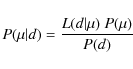
The relative position of the radio and NIR sources in these figures suggests that E1, E2 and E3 might be associated with B1, B2 and B3/C3. To better quantify these associations, as well as identify other possible counterparts, we have used Bayesian inference to calculate the probability that the compact radio sources are physically associated with their nearest optical/NIR sources. The mathematical expression of this probability has been derived as follows.
Lets ![]() be the probability density of the true distance
be the probability density of the true distance
![]() between two sources given an observed distance
d. Following Bayesian inference, this probability
is given by:
between two sources given an observed distance
d. Following Bayesian inference, this probability
is given by:
|
(1) |
where
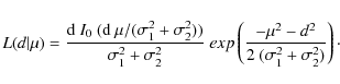
As pointed out in Churchman
et al. (2006), the likelihood of the observed
distance between two sources which positions are described by a
Gaussian distribution is not Gaussian. Instead, this likelihood in two
dimensions is given by:
|
(2) |
Where
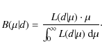
Since the area inside an annulus at radius ![]() increases as
increases as ![]() d
d![]() ,
we assume that, for a source located at a random position,
,
we assume that, for a source located at a random position,
![]() .
Therefore:
.
Therefore:
| (3) |
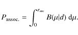
Which normalized gives:
|
(4) |
The integral of this function between
|
(5) |
A list with the nearest optical/NIR sources of each radio detection, together with their associated probabilities, is presented in Table 4. As expected, only the images of ERO B have a non-negligible probability of being associated with some of the radio sources (E1, E2 and E3). However, if E1, E2 and E3 are indeed the radio counterparts of B1, B2 and B3, they have to be multiple images produced by a radio source at
Table 4: Conunterparts of the radio detections.
![\begin{figure}
\par\includegraphics[width=8.8cm,angle=0,clip]{12903fg9.ps}
\end{figure}](/articles/aa/full_html/2010/01/aa12903-09/img206.png)
|
Figure 9:
Detail of the HST image in the region of RJ, including the critical
curve at z=2.911 predicted by the lens model
describe in Sect. 4.1
(black line). The contours correspond to the |
| Open with DEXTER | |
Finally, note that no optical/NIR counterpart has been identified with RJ. Therefore, given the depths of the optical and NIR images, it seems more likely that the extended morphology of RJ corresponds to an AGN rather than a resolved low redshift star forming galaxy. Within the AGN scenario, we expect that the peak of the radio emission corresponds to the position of an undetected optical source, and the extensions in opposite directions are two jets coming from it. Another conceivable scenario would be that the galaxy G14 is an AGN host with a one sided radio extension. However, the mayor axes of RJ does not seem to be aligned with G14, and this kind of AGN is not very common.
4.2 Comparison between radio and sub-mm
![\begin{figure}
\par\includegraphics[width=17cm,angle=0,clip]{12903fg10.ps}
\end{figure}](/articles/aa/full_html/2010/01/aa12903-09/img207.png)
|
Figure 10:
Detail of the HST image of the cluster center, with the sub-mm
850 |
| Open with DEXTER | |
In this section, we will use the FIR-radio correlation to check
whether the radio detections could be associated with the observed
sub-mm emission. To make this kind of analysis, it is necessary to
match the resolutions of the radio and sub-mm observations. Therefore,
the A+B array data was tapered with a Gaussian of
![]()
![]() and restored with a clean beam of
and restored with a clean beam of
![]() at the end of the imaging process. The
left panel of Fig. 10
shows the final tapered radio
map (white contours) superimposed upon the sub-mm map (black contours)
and the HST image of the cluster core. The positions of the detections
in the high resolution radio map have been indicated with crosses as
reference.
at the end of the imaging process. The
left panel of Fig. 10
shows the final tapered radio
map (white contours) superimposed upon the sub-mm map (black contours)
and the HST image of the cluster core. The positions of the detections
in the high resolution radio map have been indicated with crosses as
reference.
If all the observed sub-mm emission would be produced by a
single SMG
that does not host an AGN, it is expected that the radio and sub-mm
morphologies would resemble each other. This is because the origin of
the FIR-radio correlation seems to be linked to massive star
formation![]() , which means
that both the radio and sub-mm emission are originated in
(approximately) the same regions of the galaxy. However, the
, which means
that both the radio and sub-mm emission are originated in
(approximately) the same regions of the galaxy. However, the ![]() flux ratio observed in sub-mm galaxies
displays a broad scatter which strongly depends on the characteristic
dust temperature and the redshift (e.g. Blain et al. 2002; Chapman
et al. 2005). Therefore, if the observed sub-mm
emission is being produced
by several blended SMGs, we might find ``morphological
inconsistencies'' like the one present in the left panel of
Fig. 10
(note that the brightest peak of the radio
emission is located in the region of RJ instead of been coincident
with the brightest sub-mm peak).
flux ratio observed in sub-mm galaxies
displays a broad scatter which strongly depends on the characteristic
dust temperature and the redshift (e.g. Blain et al. 2002; Chapman
et al. 2005). Therefore, if the observed sub-mm
emission is being produced
by several blended SMGs, we might find ``morphological
inconsistencies'' like the one present in the left panel of
Fig. 10
(note that the brightest peak of the radio
emission is located in the region of RJ instead of been coincident
with the brightest sub-mm peak).
Interestingly, if the CC model of RJ is subtracted from the data, the morphology of the radio emission becomes remarkably similar to the sub-mm emission (right panel of Fig. 10). This result strongly suggests that the source/sources responsible for the radio emission observed in this panel are also responsible for the bulk of the sub-mm emission. The other conclusion derived from this comparison is that, if RJ is contributing to the sub-mm emission, either its properties (redshift and/or dust temperature) are different from the properties of the source/sources associated with the other radio detections, or it has a ``radio excess'' due to an AGN.
Using ![]() ,
,
![]() and 1.4 GHz observations of 15 bright SMGs
with spectroscopic redshifts, Kovács
et al. (2006) (K06
hereafter) conclude that the FIR-radio correlation remains valid for
SMGs with
and 1.4 GHz observations of 15 bright SMGs
with spectroscopic redshifts, Kovács
et al. (2006) (K06
hereafter) conclude that the FIR-radio correlation remains valid for
SMGs with ![]() and luminosities between
and luminosities between ![]() (except when they are radio-loud AGN). To
see how our system compares with this sample, we have made a more
quantitative analysis of the FIR-radio correlation using the
(except when they are radio-loud AGN). To
see how our system compares with this sample, we have made a more
quantitative analysis of the FIR-radio correlation using the ![]() parameter introduced in K06:
parameter introduced in K06:
![\begin{displaymath}q_{\rm L}= \log \left(\frac{ L_{\rm FIR}}{ [{\rm 4.52~THz}]~ L_{\rm
1.4~GHz}} \right)
\end{displaymath}](/articles/aa/full_html/2010/01/aa12903-09/img215.png)
|
(6) |
were total FIR luminosity is inferred from the flux density at
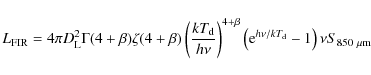
|
(7) |
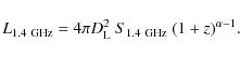
and the radio luminosity can be derived as:
|
(8) |
In these formulas,
At the position of the sub-mm peak, the radio and sub-mm
fluxes were
derived using the area delimited by the ![]() radio contour shown
in the left panel of Fig. 10 (
radio contour shown
in the left panel of Fig. 10 (
![]() mJy
and
mJy
and ![]()
![]() Jy). The
different values of
Jy). The
different values of ![]() derived from these fluxes as function
of redshift and
derived from these fluxes as function
of redshift and ![]() are shown in Fig. 11.
The
horizontal dashed lines indicate the minimum and maximum value of
are shown in Fig. 11.
The
horizontal dashed lines indicate the minimum and maximum value of
![]() found in the
K06 sample (discarding AGN hosts). Note that
there is a wide range of z and
found in the
K06 sample (discarding AGN hosts). Note that
there is a wide range of z and ![]() for which the observed
fluxes are consistent with K06. If we now assume that the radio and
sub-mm emission are produced by a (lensed) star forming galaxy at z=2.9,
only temperatures between
for which the observed
fluxes are consistent with K06. If we now assume that the radio and
sub-mm emission are produced by a (lensed) star forming galaxy at z=2.9,
only temperatures between ![]() 20-40 K
would be allowed,
which is the temperature range in which most of the K06 sources lie.
20-40 K
would be allowed,
which is the temperature range in which most of the K06 sources lie.
Since AGNs do not follow the FIR-radio correlation, an
estimate of the
![]() value for RJ
could provide extra evidence to
confirm/discard the possible AGN nature of this source. However, that
would require a higher resolution
value for RJ
could provide extra evidence to
confirm/discard the possible AGN nature of this source. However, that
would require a higher resolution ![]() map, to confirm the
connection of RJ with a discrete sub-mm source and get an accurate
estimate of its sub-mm flux. In addition, the redshift of RJ needs to
be determined in order to break the degeneracy between z
and
map, to confirm the
connection of RJ with a discrete sub-mm source and get an accurate
estimate of its sub-mm flux. In addition, the redshift of RJ needs to
be determined in order to break the degeneracy between z
and ![]() illustrated in Fig. 11.
illustrated in Fig. 11.
Finally, is important to mention that, although the energy
output of
the majority of SMGs is dominated by star formation, about ![]() host an AGN (Alexander et al. 2005).
Therefore, even if the source
associated with RJ is an AGN, it could still be contributing to the
sub-mm emission observed in that region. Other potential contributors
to the observed sub-mm emission are indicated in the right panel of
Fig. 10.
host an AGN (Alexander et al. 2005).
Therefore, even if the source
associated with RJ is an AGN, it could still be contributing to the
sub-mm emission observed in that region. Other potential contributors
to the observed sub-mm emission are indicated in the right panel of
Fig. 10.
![\begin{figure}
\par\includegraphics[width=7cm,angle=0,clip]{12903fg11.ps}
\end{figure}](/articles/aa/full_html/2010/01/aa12903-09/img228.png)
|
Figure 11:
Change of the parameter |
| Open with DEXTER | |
![\begin{figure}
\par\includegraphics[width=13.5cm,angle=0,clip]{12903fg12.ps}
\end{figure}](/articles/aa/full_html/2010/01/aa12903-09/img229.png)
|
Figure 12: Detail of the HST image of the cluster core, indicating all the galaxies that have been included in the lens model. The sizes of the ellipses correspond to the morphological parameters listed in Table 5. The lines represent the critical curves (black) and caustics (white) predicted by the lens model at z=2.911. |
| Open with DEXTER | |
5 Gravitational lens modeling of MS0451
Table 5: Galaxy catalog for the new lens model of MS0451.
In order to investigate the possible lensed nature of the
radio
detections, we used the publicly available
LENSTOOL![]() code to model the mass distribution of the cluster. This
modeling involves an optimization procedure, aimed to find the
mass model parameter values that best reproduce the observational
constrains (positions of the multiply imaged systems). For a detailed
description of the strong lensing methodology followed in the LENSTOOL
software we refer to Limousin
et al. (2007),
Jullo et al. (2007)
and the appendix A2 of Smith
et al. (2005).
code to model the mass distribution of the cluster. This
modeling involves an optimization procedure, aimed to find the
mass model parameter values that best reproduce the observational
constrains (positions of the multiply imaged systems). For a detailed
description of the strong lensing methodology followed in the LENSTOOL
software we refer to Limousin
et al. (2007),
Jullo et al. (2007)
and the appendix A2 of Smith
et al. (2005).
The current best lens model of the cluster MS0451, published
in B04
(B04 model hereafter), was produced with the first version of LENSTOOL
(Kneib et al. 1993).
This version is based on a
downhill ![]() minimization (which can be very sensitive to local
minimum in the likelihood distribution), and does not provide
estimates of the errors on the optimized parameters. The latest LENSTOOL
version (Jullo et al. 2007)
used in this paper
includes a Bayesian Monte Carlo Markov chain optimization routine,
which allows to determine errors in the optimized parameters and
lowers the probability of ending in local
minimization (which can be very sensitive to local
minimum in the likelihood distribution), and does not provide
estimates of the errors on the optimized parameters. The latest LENSTOOL
version (Jullo et al. 2007)
used in this paper
includes a Bayesian Monte Carlo Markov chain optimization routine,
which allows to determine errors in the optimized parameters and
lowers the probability of ending in local ![]() minimum.
minimum.
5.1 Mass model
![\begin{figure}
\par\includegraphics[width=7.5cm,angle=0,clip]{12903fg13.ps}
\end{figure}](/articles/aa/full_html/2010/01/aa12903-09/img232.png)
|
Figure 13: Detail of the optical arc as seeing in the HST image. The circles indicate the positions of the three sets of mirror images listed in Table 6. |
| Open with DEXTER | |
|
(9) |
The galaxy-scale component contains the cluster members located relatively close to the area were the multiple images are formed, because they are the ones that have the strongest effect in the potential of that region. We also included some fainter galaxies located close to the strong lensing constraints, since they are known to perturb the strong lensing configuration (Meneghetti et al. 2007). The details of our galaxy catalog are listed in Table 5, and their positions and sizes are displayed in Fig. 12. Note that the galaxy catalog used in the B04 model (39 galaxies in total) includes cluster members located farther away, but not the faint galaxies mentioned before.
Table 6: Constraints for the new lens model of MS0451.
5.2 Multiple images
Figure 13 shows a close up of ARC1 as seeing on the ACS image. From its knotted structure we can identify 3 sets of mirror images, each of which should have its own counter-image. However, since it is not possible to distinguish the different knots in the de-magnified image of the arc (ARC1 ci, see Fig. 14), we assigned the same position to the counter-image of each set of constraints coming from the arc.
The positions for the EROs used in our model come from the
Subaru K' band image published in Takata et al. (2003),
which is deeper and has higher
resolution than the CFHT K' band image
published by B04. Based on
their model, B04 identified the NIR source labeled B3/C3 as the result
of the blending between the counter-images of B and C. However, we
have detected a faint source (labeled ``5.3'' in Fig. 14)
located very close to B3/C3 in the Subaru K' band
image. This source
was not reported in Takata
et al. (2003) because it is too faint to be
classified as a DRG![]() (Tadafumi Takata, private
communication). Since it is possible that this source is the resolved
counter-image of ERO C, we decided to include it as a
constraint in
the new model. The full set of constraints used for the optimization
is listed in Table 6.
(Tadafumi Takata, private
communication). Since it is possible that this source is the resolved
counter-image of ERO C, we decided to include it as a
constraint in
the new model. The full set of constraints used for the optimization
is listed in Table 6.
5.3 Optimization
The set of free parameters used during the optimization are:
(i) all
the parameters that characterize the cluster halo (except ![]() )
and (ii) the velocity dispersion (
)
and (ii) the velocity dispersion (
![]() )
and
scale radius (
)
and
scale radius (
![]() )
of a galaxy at
)
of a galaxy at ![]() with a typical luminosity
with a typical luminosity ![]() that corresponds
to an observed magnitude of m=18.8.
that corresponds
to an observed magnitude of m=18.8.
The ![]() and
and ![]() of all the galaxy halos included in
the mass model are derived from the luminosity of their associated
galaxy using the following empirical scaling relations:
of all the galaxy halos included in
the mass model are derived from the luminosity of their associated
galaxy using the following empirical scaling relations:
|
(10) |
The scaling relation for
The ranges in which the free parameters are allowed to vary during the optimization are listed in Table 7. Note that the scale radius describes the properties of the mass distribution on scales much larger than the radius over which the multiple images can be found. Therefore, since strong lensing cannot give any reliable constrains on this parameter, its value is set to an arbitrary large number (1500 kpc). The ranges adopted for the L* galaxy are motivated by galaxy-galaxy lensing studies in clusters (Limousin et al. 2007; Natarajan et al. 2002b,1998,2002a).
![\begin{figure}
\par\includegraphics[width=7.5cm,angle=0,clip]{12903fg14.ps}
\end{figure}](/articles/aa/full_html/2010/01/aa12903-09/img244.png)
|
Figure 14:
Detail of the source E3, including its radio contours as presented in
Fig. 4.
Top panel: HST image of the region, including
the positions of the counter images of the optical arc (ARC1 ci) and
the ERO pair (B3/C3) reported by Borys
et al. (2004). Bottom panel: K' band
image of the region, indicating the constraints used in the lens model
(4.3 and 5.3). The radius of the circles show the estimated positional
uncertainties: |
| Open with DEXTER | |
Table 7: Ranges in which the free parameters are allowed to vary during the lens model optimization.
Table 8: Most likely mass model parameters.
Table 9: Best mass model.
Since the redshift of the EROs has not been confirmed
spectroscopically, the modeling procedure was carried out in four
steps. In the first step, only the sets of images from ARC1 at ![]() where used as constraints in the optimization. The
resultant best model was then re-optimized, including the constraints
provided by ERO B but leaving
where used as constraints in the optimization. The
resultant best model was then re-optimized, including the constraints
provided by ERO B but leaving ![]() as free parameter. As a
result, the predicted redshift of ERO B is
as free parameter. As a
result, the predicted redshift of ERO B is ![]() .
In the third step, the constraints from ERO C were used in a
new
re-optimization of the best model obtained in the previous step,
assuming
.
In the third step, the constraints from ERO C were used in a
new
re-optimization of the best model obtained in the previous step,
assuming ![]() and leaving
and leaving ![]() as free parameter. This
provides a
as free parameter. This
provides a ![]() ,
which is the same redshift that
B04 derived for the ERO pair. In the final step, the previous best
model is re-optimized (in the image plane)
including all the
constraints with z=2.911.
,
which is the same redshift that
B04 derived for the ERO pair. In the final step, the previous best
model is re-optimized (in the image plane)
including all the
constraints with z=2.911.
The Bayesian MCMC optimization routine included in the new version of LENSTOOL provides two kinds of outputs: (i) the likelihood of reproducing the observed constraints, independently derived for each free parameter of the mass model, and (ii) the set of model parameters that provides the best fit to the input data. The most likely values for the model parameters obtained from these histograms are listed in Table 8, whereas the parameters of the best model (MFINAL hereafter) are listed in Table 9.
The image positions are well reproduced, with image plane
positional
rms differences between ![]()
![]() and
and ![]() (see Table 10).
The projected mass within the Einstein
radius (here approximated by the ARC1 distance from the center, is
(see Table 10).
The projected mass within the Einstein
radius (here approximated by the ARC1 distance from the center, is
![]() .
.
5.4 Analysis of the radio data using the new lens model
![\begin{figure}
\par\includegraphics[width=17.5cm,angle=0,clip]{12903fg15.ps}
\end{figure}](/articles/aa/full_html/2010/01/aa12903-09/img261.png)
|
Figure 15:
Analisis of the lensing nature of E1, E2 and E3 with the lens model MFINAL.
The orange circles indicate the image positions predicted after tracing
each of the three radio sources independently into the source plane and
lens them back into the image plane. The radius of the circles
correspond to |
| Open with DEXTER | |
Since CR1 and CR2 are located in a region with several multiply-imaged
systems (see Fig. 8),
it is conceivable that they might
also constitute a set of mirror images. To test this hypothesis, we
redo the optimization using the positions of these two radio sources
as an additional set of constraints (system 6, see Table 6), first
assuming ![]() and then
considering
and then
considering ![]() as a free parameter. A summary of the
properties of the resultant best models (MZFIX
and MZFREE hereafter) is presented in
Tables 10
and 11.
as a free parameter. A summary of the
properties of the resultant best models (MZFIX
and MZFREE hereafter) is presented in
Tables 10
and 11.
The optimization with z free results in a
predicted redshift for
system 6 of ![]() ,
which is not consistent with
z=2.911. If we compare the probability of
MZFIX and MZFREE
to
reproduce the observations (the evidence, see Table 11), it
is clear that MZFREE is preferred over MZFIX.
Note also
that the rms difference between the observed and predicted image
positions for system 6 is three times worse for
MZFIX compared with MZFREE
(see Table 10).
On the other hand, the
total
,
which is not consistent with
z=2.911. If we compare the probability of
MZFIX and MZFREE
to
reproduce the observations (the evidence, see Table 11), it
is clear that MZFREE is preferred over MZFIX.
Note also
that the rms difference between the observed and predicted image
positions for system 6 is three times worse for
MZFIX compared with MZFREE
(see Table 10).
On the other hand, the
total ![]() of MZFREE for all the
optical/IR multiply imaged systems (
of MZFREE for all the
optical/IR multiply imaged systems (![]() optical, see Table 11) is
just slightly worse that the
corresponding
optical, see Table 11) is
just slightly worse that the
corresponding ![]() of MFINAL, which
means that MFINAL and MZFREE
are equally good. Note that the evidence cannot be used to
compare these two models because the number of free parameters in each
of them is different.
of MFINAL, which
means that MFINAL and MZFREE
are equally good. Note that the evidence cannot be used to
compare these two models because the number of free parameters in each
of them is different.
Therefore, unless the positional uncertainty of CR1 and CR2
could be
as large as ![]()
![]() (which seems unlikely, since the
positional error for these sources derived from the observations is
(which seems unlikely, since the
positional error for these sources derived from the observations is
![]() ),
these results indicate that the lens model
favors an scenario in which CR1 and CR2 (if assumed to be mirror
images) are produced by a radio source that is not located at the same
redshift as the optical arc. However, as discussed in
Sect. 3.2,
CR1 and CR2 seem to be two
relatively compact (
),
these results indicate that the lens model
favors an scenario in which CR1 and CR2 (if assumed to be mirror
images) are produced by a radio source that is not located at the same
redshift as the optical arc. However, as discussed in
Sect. 3.2,
CR1 and CR2 seem to be two
relatively compact (![]()
![]() )
regions of an extended (
)
regions of an extended (![]()
![]() )
radio source. Therefore, it is possible that this extended
radio emission is a multiply imaged structure produced by a source at
z=2.9, in which CR1 and CR2 are not mirror images.
Until the
structure of this extended radio emission can be robustly mapped with
deeper observations and included in the modeling process, the
posibility that CR1 and CR2 are associated with a lensed source at
redshift 2.9 remains open.
)
radio source. Therefore, it is possible that this extended
radio emission is a multiply imaged structure produced by a source at
z=2.9, in which CR1 and CR2 are not mirror images.
Until the
structure of this extended radio emission can be robustly mapped with
deeper observations and included in the modeling process, the
posibility that CR1 and CR2 are associated with a lensed source at
redshift 2.9 remains open.
Table 10: Results of the best models for each set of constraints.
Table 11: General results of the best models.
As mentioned in Sect. 4.1, the multiple images of ERO B have a non-negligible probability of being associated with the radio detections E1, E2 and E3. However, the probability that E3 and B3/C3 are associated is significantly lower than for E1-B1 and E2-B2. For this reason, we used MFINAL to check if the positions of E1, E2 and E3 would be consistent with a set of three images produced by a radio source at z=2.9. This was done in the following way: for each radio detection, its position was traced back into the source plane, and the resultant source was lensed again into the image plane. In this way, the model provided three predicted positions for each radio source, one of them being the position used as input.
The results (shown in Fig. 15) indicate that E3 cannot be interpreted as the radio counterpart of B3/C3, since the images produced by E1 and E2 in the counter image region are located on the right side of B3/C3 (unlike in the case of E1 and E2), at a distance which is inconsistent with the average rms of MFINAL. A possible scenario that can explain this result is that E1 and E2 are multiple images (but we don't detect the associated counter-image because it is too faint) and E3 is a non-lensed radio galaxy that it is serendipitously lying in this region. However, as it will be discussed in the next section, it is also possible to explain E3 as a lensed image produced by a source at z=2.9 under the merger scenario proposed in B04.
6 Discussion: the merger scenario
Figure 8 shows a detail of the HST image at the position of the sub-mm peak, where ARC1 and the EROs are located. The contour map of the right panel indicates the total radio emission observed in this region, whereas the left and central panels show the compact and extended component. The black line correspond to the critical curve at z=2.9 predicted by the lens model of the cluster described in Sect. 5.
If ARC1 and the EROs are indeed multiple images produced by three different regions of a merger at z=2.9, the rest of the merger lying between them should also be multiply-imaged. Hence, if the merger contains a lot of dust (as expected from a high-z SMG), this images would not be seen in the optical, but they would show up in the radio.
Under this scenario, the fact that CR1 and CR2 do not seem to have optical counterparts, and lie in the region between ARC1 and the ERO images, suggests that they could be lensed images associated with the highly-obscured center of the merger. However, as discussed in Sect. 5.4, they can also be interpreted as a set of mirror images produced by another radio galaxy located at a different redshift. The real strong evidence in favor of the merger hypothesis comes from the extended component in which CR1 and CR2 seem to be embedded, which provides 38% of the observed radio flux in the region of the sub-mm peak. As is clearly shown in the central panel of Fig. 8, this extended component constitutes a bridge of emission between the compact radio sources, as expected from the multiply imaged dust-obscured material of the merger located between the optical and NIR emitting regions. In complete agreement with this scenario, the shape of the total radio emission in the right panel of Fig. 8 follows the distribution of the optical arc and the ERO images remarkably well.
In this case, we can also expect the extended emission to be multiply imaged like ARC1 and the EROs, producing a counter-image in the region between ARC1 ci and B3/C3 (see Fig. 14). Since the images in this region are de-magnified, it is likely that the expected radio counterpart of B3/C3, and the counter image associated with the extended emission, are blended. That would shift the peak of the total observed radio emission towards ARC1 ci, explaining why the probability derived for E3-B3/C3 is much lower than what it is found for E1-B1 and E2-B2.
Finally, it is also not surprising that E1-B1 and E2-B2 are
not
identified as robust (![]()
![]() )
counterpart pairs. With the cluster
magnification generating a high resolution (distorted) view of the
inner structure of the merger, the observed offset between E1-B1 and
E2-B2 could be real, indicating that the NIR and radio emissions are
arising from slightly different regions inside the merger.
)
counterpart pairs. With the cluster
magnification generating a high resolution (distorted) view of the
inner structure of the merger, the observed offset between E1-B1 and
E2-B2 could be real, indicating that the NIR and radio emissions are
arising from slightly different regions inside the merger.
7 Summary and conclusions
SMM J04542-0301 is an elongated region of bright sub-mm emission located in the core of the cluster MS0451.6-0305. It has been suggested (Borys et al. 2004) to be partially produced by a multiply-imaged z=2.9 merger which contains a LBG (lensed as ARC1 and ARC1 ci), and two EROs (lensed as B1, B2, C1, C2 and B3/C3). Given the low resolution and poor positional accuracy of the sub-mm map, it is very difficult to confirm the connection between SMM J04542-0301 and the optical/NIR lensed images. However, high resolution radio interferometric observations can help to establish this connection thanks to the FIR-radio correlation, which has being found to be valid for SMGs (Vlahakis et al. 2007; Kovács et al. 2006; Michaowski et al. 2009; Ibar et al. 2008).
In a previous paper (Berciano Alba et al. 2007), we reported on the detection of 1.4 GHz radio emission coincident with this system using VLA archival data. Now, following a more sophisticated data reduction procedure, the previous B-array observations have being re-reduced and combined with new high resolution A-array observations. The resultant data set has been used to produced two radio maps of the cluster core:
- (i)
- a deep (

 Jy), high
resolution (
Jy), high
resolution (
 )
map, to compare with the optical/NIR images. In this map we have
detected 5 sources (E1, E2, CR1, CR2 and E3) located near the
optical/NIR lensed images, and one source (RJ) located in the central
region of the sub-mm emission (see Fig. 4). Despite
the fact that some of the sources have SNR <
5, the fact that
the
)
map, to compare with the optical/NIR images. In this map we have
detected 5 sources (E1, E2, CR1, CR2 and E3) located near the
optical/NIR lensed images, and one source (RJ) located in the central
region of the sub-mm emission (see Fig. 4). Despite
the fact that some of the sources have SNR <
5, the fact that
the  peaks lie far from the central target region adds
confidence to the reality of the sources.
peaks lie far from the central target region adds
confidence to the reality of the sources.
- (ii)
- a
 resolution map, to compare with
SMM J04542-0301 (see Fig. 10).
resolution map, to compare with
SMM J04542-0301 (see Fig. 10).
On the other hand, the other five radio detections constitute a strong observational evidence in favor of the merger scenario proposed by Borys et al. (2004). The evidence that supports this conclusion can be summarized as follows:
- if the optical arc and the EROs are multiple images produced by three different regions of a merger at z=2.9, the dust obscured material between these regions is expected to be lensed in the same way, but only visible at radio and sub-mm. In agreement with this scenario, the shape of the radio emission observed at the sub-mm peak follows the distribution of the optical arc and the ERO images remarkably well (Fig. 7);
- CR1 and CR2 do not have any optical/NIR counterpart.
However, they seem to constitute two relatively compact emitting
regions embedded in a
 extended source located between E1 and E2. The presence of this
extended component (which contributes 38% of the total radio flux in
the sub-mm peak) can only be explained if it is being produced by the
dust obscured lensed material in the center of the merger;
extended source located between E1 and E2. The presence of this
extended component (which contributes 38% of the total radio flux in
the sub-mm peak) can only be explained if it is being produced by the
dust obscured lensed material in the center of the merger;
- the compact sources E1 and E2 have a high probability of being associated with the images of ERO B, but this probability is considerably lower for E3-B3/C3. A plausible explanation of this result can be provided by the merger scenario, in which the lensed extended component is expected to have a counter image which would be blended with the radio emission associated with E3/C3. This would shift the position of the total observed peak, lowering the probability of identifying E3 and B3/C3 as counterparts;
- the fact that B1, B2 and B3/C3 are not robust (

 )
counterparts of E1, E2 and E3, indicates that the radio and NIR
emission is being produced at slightly different positions in the
sources plane, which can be distinguished thanks to the enhanced
resolution provided by the lensing magnification;
)
counterparts of E1, E2 and E3, indicates that the radio and NIR
emission is being produced at slightly different positions in the
sources plane, which can be distinguished thanks to the enhanced
resolution provided by the lensing magnification;
- if the
resolution radio map is produced after the CC model of RJ is subtracted
from the data, its morphology turns out to be remarkably similar to the
sub-mm map (right panel of Fig. 10). This
result strongly suggests that the sources E1, E2, CR1, CR2 and E3 are
associated with the extended sub-mm emission, allowing us to establish
a direct link between SMM J04542-0301 and the merger.
Including the positions of CR1 and CR2 as mirror images in the model significantly degrades the overall rms of the optimization. However, since these two sources are embedded in an extended source (which cannot be included in the lens model due to the current limitations of the LENSTOOL code), it is very difficult to establish a one-to-one identification of structures in the image plane. Therefore, the possibility that CR1 and CR2 are lensed images produced by the dust-obscured core of the merger remains open.
8 Future prospects
Radio observations of SMGs have been traditionally used to identify their optical/NIR counterparts, but also to provide estimates of their sizes (Biggs & Ivison 2008; Chapman et al. 2004). On the other hand, the magnification bias due to the gravitational lensing effect produced by clusters of galaxies has been used to increase the detection rate in sub-mm surveys, and constrain the faint flux end of the submm counts (e.g. Knudsen et al. 2008). The observations presented in this paper, however, illustrate that the prospects for both radio interferometry and strong gravitational lensing in clusters of galaxies to study the internal structure of sub-mm galaxies (SMGs) are also very promising. With the improved sensitivity of e-MERLIN and EVLA, and the revolutionary view of the sub-mm sky that will be provided by ALMA, the enhanced resolution of multiply-imaged submm galaxies might permit us, among other things, to resolve for the first time their different star-forming regions, and help to assess the connection between starburst and AGN processes that seem to coexist in these systems.
SMM04542-0301 constitutes a very promising system to carry out
this
kind of studies, but there is still one fundamental piece of
information that is missing: redshift information for the NIR, radio
and submm components. Current millimeter facilities can provide
redshift information by detecting (for instance) CO rotational lines,
but the relatively narrow bandwidths of their receivers
(<10 GHz
compared with the 115 GHz spacing between CO rotational lines) makes
the search of multiple lines very time consuming, and a prior estimate
of the redshift of the source is required. Fortunately, blind
CO redshift observations are now possible thanks to Z-Spec, a
broadband
(![]() 115 GHz)
millimeter/sub-millimeter spectrograph that has been
commissioned at the 10.4-m Caltech Submillimeter Observatory
(Bradford et al. 2009).
Once all the sources that are contributing to the
observed sub-mm emission of SMM04542-0301 have been robustly
identified, the increased bandwidth and sensitivity of the new
receivers that have been installed on the IRAM
115 GHz)
millimeter/sub-millimeter spectrograph that has been
commissioned at the 10.4-m Caltech Submillimeter Observatory
(Bradford et al. 2009).
Once all the sources that are contributing to the
observed sub-mm emission of SMM04542-0301 have been robustly
identified, the increased bandwidth and sensitivity of the new
receivers that have been installed on the IRAM![]() 30 m telescope (located on the Pico
Veleta, Spain) and the Plateau de Bure Interferometer (located in the
French Alps), will be well placed to characterize the physical
properties of this system in detail.
30 m telescope (located on the Pico
Veleta, Spain) and the Plateau de Bure Interferometer (located in the
French Alps), will be well placed to characterize the physical
properties of this system in detail.
Finally note that, since these kind of systems consist of multiple distorted images of the lensed object, a reliable reconstruction of the source is essential for their interpretation. Therefore, to be able to follow this line of research, the technological development in the observational side has to be accompanied by a similar development in the lens modeling techniques in clusters of galaxies, to properly account for the extra complexities associated with extended emission and interferometric observations.
AcknowledgementsThe authors wish to thank Sean Moran and Tadafumi Takata for providing the HST and SUBARU images and source catalogs to compare with the radio observations, and J.P. Kneib for providing the previous LENSTOOL model on MS0451. We are also very grateful to the anonymous referee for his/her useful comments and positive feedback about the paper.
A.B.A. would like to thank Christian Struve and Tom Oosterloo for discussions and helpfull insights regarding the radio data reduction and analysis, Oliver Czoske for helping with the alignment of the different maps and Simona Vegetti for the useful discussions about the lens model (which significantly improved the presentation of the model results). A special mention is reserved for Edo Loenen and Ger de Bruyn, for their crucial contribution in the analysis and interpretation.
This work was supported by the European Community's Sixth Framework Marie Curie Research Training Network Programme, Contract No. MRTN-CT-2004-505183 ``ANGLES''. O.W. was funded by ANGLES and by the Emmy-Noether-Programme of the Deutsche Forschungemeinschaft, reference Wu 588/1-1. M.L. acknowledges the Centre National d'Études Spatiales (CNES) for their support. The Dark Cosmology Centre is funded by the Danish National Research Foundation.
References
- Alexander, D. M., Bauer, F. E., Brandt, W. N., et al. 2003, AJ, 126, 539 [NASA ADS] [CrossRef] [Google Scholar]
- Alexander, D. M., Bauer, F. E., Chapman, S. C., et al. 2005, ApJ, 632, 736 [NASA ADS] [CrossRef] [Google Scholar]
- Appleton, P. N., Fadda, D. T., Marleau, F. R., et al. 2004, ApJS, 154, 147 [NASA ADS] [CrossRef] [Google Scholar]
- Barger, A. J., Cowie, L. L., Sanders, D. B., et al. 1998, Nature, 394, 248 [NASA ADS] [CrossRef] [Google Scholar]
- Barger, A. J., Cowie, L. L., & Richards, E. A. 2000, AJ, 119, 2092 [Google Scholar]
- Beelen, A., Cox, P., Benford, D. J., et al. 2006, ApJ, 642, 694 [NASA ADS] [CrossRef] [Google Scholar]
- Berciano Alba, A., Garrett, M. A., Koopmans, L. V. E., & Wucknitz, O. 2007, A&A, 462, 903 [Google Scholar]
- Biggs, A. D., & Ivison, R. J. 2008, MNRAS, 385, 893 [NASA ADS] [CrossRef] [Google Scholar]
- Blain, A. W., & Longair, M. S. 1993, MNRAS, 264, 509 [NASA ADS] [CrossRef] [Google Scholar]
- Blain, A. W., Smail, I., Ivison, R. J., Kneib, J.-P., & Frayer, D. T. 2002, Phys. Rep., 369, 111 [NASA ADS] [CrossRef] [Google Scholar]
- Borys, C., Chapman, S., Donahue, M., et al. 2004, MNRAS, 352, 759 (B04) [NASA ADS] [CrossRef] [Google Scholar]
- Bradford, C. M., Aguirre, J. E., Aikin, R., et al. 2009, ApJ, 705, 112 [NASA ADS] [CrossRef] [Google Scholar]
- Chapman, S. C., Scott, D., Borys, C., & Fahlman, G. G. 2002, MNRAS, 330, 92 [NASA ADS] [CrossRef] [Google Scholar]
- Chapman, S. C., Smail, I., Windhorst, R., Muxlow, T., & Ivison, R. J. 2004, ApJ, 611, 732 [NASA ADS] [CrossRef] [Google Scholar]
- Chapman, S. C., Blain, A. W., Smail, I., & Ivison, R. J. 2005, ApJ, 622, 772 [NASA ADS] [CrossRef] [Google Scholar]
- Churchman, L. S., Flyvbjerg, H., & Spudich, J. A. 2006, Biophys. J., 90, 668 [CrossRef] [PubMed] [Google Scholar]
- Condon, J. J., Condon, M. A., Gisler, G., & Puschell, J. J. 1982, ApJ, 252, 102 [NASA ADS] [CrossRef] [Google Scholar]
- Cowie, L. L., Barger, A. J., & Kneib, J.-P. 2002, AJ, 123, 2197 [NASA ADS] [CrossRef] [Google Scholar]
- Eales, S., Lilly, S., Gear, W., et al. 1999, ApJ, 515, 518 [NASA ADS] [CrossRef] [Google Scholar]
- Elíasdóttir, Á., Limousin, M., Richard, J., et al. 2007, ArXiv e-prints [Google Scholar]
- Franceschini, A., Toffolatti, L., Mazzei, P., Danese, L., & de Zotti, G. 1991, A&AS, 89, 285 [Google Scholar]
- Garrett, M. A. 2002, A&A, 384, L19 [Google Scholar]
- Garrett, M. A., Knudsen, K. K., & van der Werf, P. P. 2005, A&A, 431, L21 [Google Scholar]
- Genzel, R., Baker, A. J., Tacconi, L. J., et al. 2003, ApJ, 584, 633 [NASA ADS] [CrossRef] [Google Scholar]
- Greve, T. R., Bertoldi, F., Smail, I., et al. 2005, MNRAS, 359, 1165 [NASA ADS] [CrossRef] [Google Scholar]
- Hauser, M. G., Arendt, R. G., Kelsall, T., et al. 1998, ApJ, 508, 25 [NASA ADS] [CrossRef] [Google Scholar]
- Helou, G., Soifer, B. T., & Rowan-Robinson, M. 1985, ApJ, 298, L7 [Google Scholar]
- Hughes, D. H., Serjeant, S., Dunlop, J., et al. 1998, Nature, 394, 241 [NASA ADS] [CrossRef] [Google Scholar]
- Ibar, E., Cirasuolo, M., Ivison, R., et al. 2008, MNRAS, 386, 953 [NASA ADS] [CrossRef] [Google Scholar]
- Ivison, R. J., Smail, I., Barger, A. J., et al. 2000, MNRAS, 315, 209 [NASA ADS] [CrossRef] [Google Scholar]
- Ivison, R. J., Greve, T. R., Dunlop, J. S., et al. 2007, MNRAS, 380, 199 [Google Scholar]
- Jullo, E., Kneib, J.-P., Limousin, M., et al. 2007, New J. Phys., 9, 447 [Google Scholar]
- Kettenis, M., van Langevelde, H. J., Reynolds, C., & Cotton, B. 2006, in Astronomical Data Analysis Software and Systems XV, ed. C. Gabriel, C. Arviset, D. Ponz, & S. Enrique, ASP Conf. Ser., 351, 497 [Google Scholar]
- Kneib, J. P., Mellier, Y., Fort, B., & Mathez, G. 1993, A&A, 273, 367 [Google Scholar]
- Kneib, J.-P., van der Werf, P. P., Kraiberg Knudsen, K., et al. 2004, MNRAS, 349, 1211 [NASA ADS] [CrossRef] [Google Scholar]
- Kneib, J.-P., Neri, R., Smail, I., et al. 2005, A&A, 434, 819 [Google Scholar]
- Knudsen, K. K., van der Werf, P. P., & Kneib, J.-P. 2008, MNRAS, 384, 1611 [NASA ADS] [CrossRef] [Google Scholar]
- Knudsen, K. K., Neri, R., Kneib, J.-P., & van der Werf, P. P. 2009, A&A, 496, 45 [Google Scholar]
- Kodama, T., Tanaka, M., Tamura, T., et al. 2005, PASJ, 57, 309 [NASA ADS] [Google Scholar]
- Kovács, A., Chapman, S. C., Dowell, C. D., et al. 2006, ApJ, 650, 592 [NASA ADS] [CrossRef] [Google Scholar]
- Lagache, G., Puget, J.-L., & Dole, H. 2005, ARA&A, 43, 727 [Google Scholar]
- Lilly, S. J., Eales, S. A., Gear, W. K. P., et al. 1999, ApJ, 518, 641 [NASA ADS] [CrossRef] [Google Scholar]
- Limousin, M., Kneib, J.-P., & Natarajan, P. 2005, MNRAS, 356, 309 [NASA ADS] [CrossRef] [Google Scholar]
- Limousin, M., Richard, J., Jullo, E., et al. 2007, ApJ, 668, 643 [NASA ADS] [CrossRef] [Google Scholar]
- Lonsdale, C. J., Farrah, D., & Smith, H. E. 2006, Ultraluminous Infrared Galaxies (Astrophysics Update 2), 285 [Google Scholar]
- Meneghetti, M., Bartelmann, M., Jenkins, A., & Frenk, C. 2007, MNRAS, 381, 171 [NASA ADS] [CrossRef] [Google Scholar]
- Micha▯owski, M. J., Hjorth, J., & Watson, D. 2009, ArXiv e-prints [Google Scholar]
- Moran, S. M., Ellis, R. S., Treu, T., et al. 2007, ApJ, 671, 1503 [NASA ADS] [CrossRef] [Google Scholar]
- Natarajan, P., Kneib, J.-P., Smail, I., & Ellis, R. S. 1998, ApJ, 499, 600 [NASA ADS] [CrossRef] [Google Scholar]
- Natarajan, P., Kneib, J.-P., & Smail, I. 2002a, ApJ, 580, L11 [NASA ADS] [CrossRef] [Google Scholar]
- Natarajan, P., Loeb, A., Kneib, J.-P., & Smail, I. 2002b, ApJ, 580, L17 [NASA ADS] [CrossRef] [Google Scholar]
- Neri, R., Genzel, R., Ivison, R. J., et al. 2003, ApJ, 597, L113 [NASA ADS] [CrossRef] [Google Scholar]
- Puget, J.-L., Abergel, A., Bernard, J.-P., et al. 1996, A&A, 308, L5 [Google Scholar]
- Smail, I., Ivison, R. J., & Blain, A. W. 1997, ApJ, 490, L5 [NASA ADS] [CrossRef] [Google Scholar]
- Smail, I., Ivison, R. J., Blain, A. W., & Kneib, J.-P. 2002, MNRAS, 331, 495 [NASA ADS] [CrossRef] [Google Scholar]
- Smail, I., Chapman, S. C., Blain, A. W., & Ivison, R. J. 2004, ApJ, 616, 71 [NASA ADS] [CrossRef] [Google Scholar]
- Smith, G. P., Kneib, J.-P., Smail, I., et al. 2005, MNRAS, 359, 417 [NASA ADS] [CrossRef] [Google Scholar]
- Spergel, D. N., Bean, R., Doré, O., et al. 2007, ApJS, 170, 377 [NASA ADS] [CrossRef] [Google Scholar]
- Swinbank, A. M., Chapman, S. C., Smail, I., et al. 2006, MNRAS, 371, 465 [NASA ADS] [CrossRef] [Google Scholar]
- Swinbank, A. M., Bower, R. G., Smith, G. P., et al. 2007, MNRAS, 376, 479 [NASA ADS] [CrossRef] [Google Scholar]
- Tacconi, L. J., Neri, R., Chapman, S. C., et al. 2006, ApJ, 640, 228 [NASA ADS] [CrossRef] [Google Scholar]
- Takata, T., Kashikawa, N., Nakanishi, K., et al. 2003, PASJ, 55, 789 (T03) [NASA ADS] [Google Scholar]
- van der Kruit, P. C. 1971, A&A, 15, 110 [Google Scholar]
- Vlahakis, C., Eales, S., & Dunne, L. 2007, MNRAS, 379, 1042 [NASA ADS] [CrossRef] [Google Scholar]
- Wang, W.-H., Cowie, L. L., van Saders, J., Barger, A. J., & Williams, J. P. 2007, ApJ, 670, L89 [NASA ADS] [CrossRef] [Google Scholar]
- Webb, T. M. A., Lilly, S. J., Clements, D. L., et al. 2003, ApJ, 597, 680 [NASA ADS] [CrossRef] [Google Scholar]
Footnotes
- ... SCUBA
![[*]](/icons/foot_motif.png)
- Submillimeter Common-User Bolometer Array, decommissioned in September 2005 from the James Clerk Maxwell Telescope on Mauna Kea.
- ...
EROs
- Extremely Red Objects, photometrically defined as R-K > 5.3.
- ... VLA
- Very Large Array interferometer of the National Radio Astronomy Observatory (NRAO).
- ...
sources
- The NRAO VLA Sky Survey (NVSS) is a 1.4 GHz continuum survey covering the entire sky north of -40 deg. declination, with a completeness limit about 2.5 mJy.
- ... system
- Project ID AN0109, PI: Nakanishi.
- ...
image
- Astrometry matched to Subaru/Suprime-Cam observations of MS0451 for the PISCES survey (Kodama et al. 2005).
- ...

- Which corresponds to a clean beam of
 .
.
- ...
formation
- While young massive stars produce UV radiation that is re-emitted in the FIR by the surrounding dust, old massive stars die as SN producing electrons that are accelerated by the galactic magnetic field generating synchrotron radio emission.
- ...
LENSTOOL
- http://www.oamp.fr/cosmology/lenstool/
- ... DRG
- Distant Red Galaxies, photometrically
defined as
 .
.
- ... IRAM
- Institut de Radioastronomie Millimetrique.
All Tables
Table 1: Information about the identifyed radio sources in the core of MS0451.
Table 2: Gaussian fitting results for the identified compact radio sources in the core of MS0451.
Table 3: Observations details.
Table 4: Conunterparts of the radio detections.
Table 5: Galaxy catalog for the new lens model of MS0451.
Table 6: Constraints for the new lens model of MS0451.
Table 7: Ranges in which the free parameters are allowed to vary during the lens model optimization.
Table 8: Most likely mass model parameters.
Table 9: Best mass model.
Table 10: Results of the best models for each set of constraints.
Table 11: General results of the best models.
All Figures
|
|
Figure 1:
Summary of the results presented in
Borys et al. (2004).
SCUBA |
| Open with DEXTER | |
| In the text | |
|
|
Figure 2:
VLA 1.4 GHz maps centered in the core of the cluster
MS0451.6-0305. The maps were produced using the visibilities of the
central 10
|
| Open with DEXTER | |
| In the text | |
|
|
Figure 3: Histogram of the A+B array clean map produced using R=0.6. The black curve is the best Gaussian fit to the noise peak, while the positive excess on the right side is due to source emission. The good agreement between the fit and the data in the negative side of the Gaussian indicates that the noise of the map is well behaved, making faint detections more reliable. |
| Open with DEXTER | |
| In the text | |
|
|
Figure 4:
VLA 1.4 GHz map derived from the A+B-array data set using
R=0.6. The greyscale has units of Jy beam-1,
and the
corresponding contours (white) are drawn at -4, 4, 5, 6, 8,
10, 14,
18, 28, 48 and 78 times the 1 |
| Open with DEXTER | |
| In the text | |
|
|
Figure 5:
Detail of the six radio sources located within the sub-mm
emission region in Fig. 4. The white
radio contours
are drawn at 2, 3, 4, 5, 6 and 8 times the 1 |
| Open with DEXTER | |
| In the text | |
|
|
Figure 6: Detail of Fig. 4. The grey scale has been modified to make more evident the low level background in this region of the radio map. |
| Open with DEXTER | |
| In the text | |
|
|
Figure 7:
VLA 1.4 GHz maps obtained by tapering the A+B-array data set
with a Gaussian of |
| Open with DEXTER | |
| In the text | |
|
|
Figure 8:
Detail of the HST image in the arc region, including the critical curve
at z=2.911 predicted by the lens model described in
Sect. 5
(black line). The red circles indicate the positions of the multiply
imaged EROs mentioned in Borys
et al. (2004), whereas the blue circles correspond
to the compact radio detections indentified in this region. The radius
of the circles indicate the estimated positional errors: |
| Open with DEXTER | |
| In the text | |
|
|
Figure 9:
Detail of the HST image in the region of RJ, including the critical
curve at z=2.911 predicted by the lens model
describe in Sect. 4.1
(black line). The contours correspond to the |
| Open with DEXTER | |
| In the text | |
|
|
Figure 10:
Detail of the HST image of the cluster center, with the sub-mm
850 |
| Open with DEXTER | |
| In the text | |
|
|
Figure 11:
Change of the parameter |
| Open with DEXTER | |
| In the text | |
|
|
Figure 12: Detail of the HST image of the cluster core, indicating all the galaxies that have been included in the lens model. The sizes of the ellipses correspond to the morphological parameters listed in Table 5. The lines represent the critical curves (black) and caustics (white) predicted by the lens model at z=2.911. |
| Open with DEXTER | |
| In the text | |
|
|
Figure 13: Detail of the optical arc as seeing in the HST image. The circles indicate the positions of the three sets of mirror images listed in Table 6. |
| Open with DEXTER | |
| In the text | |
|
|
Figure 14:
Detail of the source E3, including its radio contours as presented in
Fig. 4.
Top panel: HST image of the region, including
the positions of the counter images of the optical arc (ARC1 ci) and
the ERO pair (B3/C3) reported by Borys
et al. (2004). Bottom panel: K' band
image of the region, indicating the constraints used in the lens model
(4.3 and 5.3). The radius of the circles show the estimated positional
uncertainties: |
| Open with DEXTER | |
| In the text | |
|
|
Figure 15:
Analisis of the lensing nature of E1, E2 and E3 with the lens model MFINAL.
The orange circles indicate the image positions predicted after tracing
each of the three radio sources independently into the source plane and
lens them back into the image plane. The radius of the circles
correspond to |
| Open with DEXTER | |
| In the text | |
Copyright ESO 2010
Current usage metrics show cumulative count of Article Views (full-text article views including HTML views, PDF and ePub downloads, according to the available data) and Abstracts Views on Vision4Press platform.
Data correspond to usage on the plateform after 2015. The current usage metrics is available 48-96 hours after online publication and is updated daily on week days.
Initial download of the metrics may take a while.