| Issue |
A&A
Volume 507, Number 2, November IV 2009
|
|
|---|---|---|
| Page(s) | 589 - 597 | |
| Section | Astrophysical processes | |
| DOI | https://doi.org/10.1051/0004-6361/200912755 | |
| Published online | 17 September 2009 | |
A&A 507, 589-597 (2009)
Analytical description of nonlinear cosmic ray scattering: isotropic and quasilinear regimes of pitch-angle diffusion
A. Shalchi - T. Skoda - R. C. Tautz - R. Schlickeiser
Institut für Theoretische Physik, Lehrstuhl IV: Weltraum- und Astrophysik, Ruhr-Universität Bochum, 44780 Bochum, Germany
Received 24 June 2009 / Accepted 21 August 2009
Abstract
Aims. We investigate pitch-angle scattering, which is a fundamental process in the physics of cosmic rays.
Methods. By employing the second-order quasilinear theory, the
pitch-angle Fokker-Planck coefficient is calculated analytically for
the first time.
Results. We demonstrate that for sufficiently strong turbulence
the pitch-angle Fokker-Planck coefficient is isotropic. The derived
results can be used to compute the parallel mean free path for all
forms of the turbulence spectrum. We also consider applications, namely
the transport of solar energetic particles and the propagation of
cosmic rays in the Galaxy.
Conclusions. The previously used assumption of isotropic
pitch-angle diffusion is indeed correct for sufficiently strong
turbulence. An analytical description of nonlinear particle scattering
is possible.
Key words: acceleration of particles - diffusion - cosmic rays - Magnetohydrodynamics (MHD) - turbulence - interplanetary medium
1 Introduction
Here, we revisit the problem of charged particle transport in MHD
turbulence. Particle transport is described by the diffusion tensor
![]() in the case of diffusive propagation. For certain parameters regimes (for a detailed discussion see Shalchi & Dosch 2009), one expects isotropic scattering. In this case the tensor is given by
in the case of diffusive propagation. For certain parameters regimes (for a detailed discussion see Shalchi & Dosch 2009), one expects isotropic scattering. In this case the tensor is given by
![]() .
In addition to the turbulent magnetic fields
.
In addition to the turbulent magnetic fields
![]() we expect
the existence of a non-vanishing mean magnetic field
we expect
the existence of a non-vanishing mean magnetic field
![]() .
The latter parameter breaks
the symmetry of the physical system leading to different diffusion
coefficients along and across the mean magnetic field. For not too
strong turbulent fields we expect
.
The latter parameter breaks
the symmetry of the physical system leading to different diffusion
coefficients along and across the mean magnetic field. For not too
strong turbulent fields we expect
![]() .
In this case the parallel spatial diffusion coefficient
.
In this case the parallel spatial diffusion coefficient
![]() controls the particle
motion.
controls the particle
motion.
An important example for the application of diffusion theory is the propagation and acceleration of charged cosmic rays (for a review see Shalchi 2009b). The investigation of these processes is relevant for different physical systems. Some examples are the solar corona (see, e.g., Fletcher 1997; Gkioulidou et al. 2007), the heliosphere (e.g., Dröge 2000; Shalchi et al. 2006; Alania & Wawrzynczak 2008), the interstellar medium (see, e.g., Yan & Lazarian 2002; Shalchi & Schlickeiser 2005), and shock waves (see, e.g., Zank et al. 2000; Li et al. 2003; Li et al. 2005; Zank et al. 2006).
The parallel mean free path
![]() of the charged particle is related to the parallel spatial diffusion coefficient
of the charged particle is related to the parallel spatial diffusion coefficient
![]() via
via
![]() and can be expressed as an integral over the inverse pitch-angle Fokker-Planck coefficient
and can be expressed as an integral over the inverse pitch-angle Fokker-Planck coefficient
![]() (see, e.g., Earl 1974)
(see, e.g., Earl 1974)
with the pitch-angle cosine
The first approach to compute the parameter
![]() was the application of perturbation theory also known as quasilinear theory (QLT, Jokipii 1966). In the years after QLT had been developed, it was noticed that
the theory is not able to describe pitch-angle scattering at
was the application of perturbation theory also known as quasilinear theory (QLT, Jokipii 1966). In the years after QLT had been developed, it was noticed that
the theory is not able to describe pitch-angle scattering at ![]() (corresponding to
(corresponding to ![]() )
correctly. This problem,
which is known as the
)
correctly. This problem,
which is known as the ![]() scattering problem, was then investigated in numerous papers (see, e.g., Jones et al. 1973; Völk 1973; Owens 1974; Völk 1975; Goldstein 1976; Jones et al. 1978).
In these
articles, QLT has been improved by replacing unperturbed orbits by more
appropriate models. However, some
of these previous theories do not provide agreement with simulations or
they are difficult to apply due to mathematical problems (see Shalchi 2009a,b). More recently, a second order quasilinear theory (SOQLT, Shalchi 2005a)
was developed. This theory is in good agreement with test-particle
simulations (for a detailed comparision between SOQLT and simulations
we refer to Shalchi 2007) and is mathematically tractable. Furthermore, Tautz et al.
(2008) have demonstrated that SOQLT can reproduce the simulations of Giacalone & Jokipii (1999) performed
for isotropic turbulence.
scattering problem, was then investigated in numerous papers (see, e.g., Jones et al. 1973; Völk 1973; Owens 1974; Völk 1975; Goldstein 1976; Jones et al. 1978).
In these
articles, QLT has been improved by replacing unperturbed orbits by more
appropriate models. However, some
of these previous theories do not provide agreement with simulations or
they are difficult to apply due to mathematical problems (see Shalchi 2009a,b). More recently, a second order quasilinear theory (SOQLT, Shalchi 2005a)
was developed. This theory is in good agreement with test-particle
simulations (for a detailed comparision between SOQLT and simulations
we refer to Shalchi 2007) and is mathematically tractable. Furthermore, Tautz et al.
(2008) have demonstrated that SOQLT can reproduce the simulations of Giacalone & Jokipii (1999) performed
for isotropic turbulence.
In previous applications of nonlinear theories for pitch-angle scattering and parallel spatial diffusion, only numerical results have been derived due to mathematical intractability. Analytical forms of these parameters are, however, very useful for different astrophysical applications. It is the purpose of the present article to investigate the SOQLT analytically for the first time. In previous articles, simple models have been used without justification. In the theory of diffusive shock acceleration, for instance, it was often assumed that pitch-angle scattering is isotropic (see, e.g., Kirk & Schneider 1988; Schneider & Kirk 1989; Kirk & Schneider 1989), in disagreement with the quasilinear result. It is also the purpose of the present article to investigate the validity of the assumption of isotropic scattering.
In Sect. 8 we consider some applications of our analytical results, namely:
- 1.
- cosmic rays from the Sun;
- 2.
- interstellar transport and steep turbulence spectra;
- 3.
- the Hillas limit and high energetic particles.
2 Standard quasilinear theory
The Fokker-Planck coefficient
![]() used in Eq. (1) can be computed by employing the so-called Taylor-Green-Kubo formulation (TGK formulation, e.g. Taylor 1922; Green 1952; Kubo 1957)
used in Eq. (1) can be computed by employing the so-called Taylor-Green-Kubo formulation (TGK formulation, e.g. Taylor 1922; Green 1952; Kubo 1957)
|
(2) |
The acceleration parameter
![\begin{displaymath}\dot{\mu} = {1 \over R_L} \left( v_x (t) \frac{\delta B_y \le...
...) \frac{\delta B_x \left[ \vec{x} (t), t \right]}{B_0} \right)
\end{displaymath}](/articles/aa/full_html/2009/44/aa12755-09/img29.png)
for purely magnetic fields
|
(4) |
with the unperturbed gyrofrequency
The simplest method to compute the parameter
![]() is the application of perturbation theory also known as quasilinear theory (Jokipii 1966). In this case the velocities vx (t) and vy (t) as well as the
particle trajectories
is the application of perturbation theory also known as quasilinear theory (Jokipii 1966). In this case the velocities vx (t) and vy (t) as well as the
particle trajectories
![]() in Eq. (3)
are replaced by the unperturbed particle orbit. A further assumption
which is often used is that the stochastic magnetic fields are replaced
by the so-called magnetostatic
slab model for which we assume
in Eq. (3)
are replaced by the unperturbed particle orbit. A further assumption
which is often used is that the stochastic magnetic fields are replaced
by the so-called magnetostatic
slab model for which we assume
![]() .
For the slab model the magnetic correlation tensor is given by
.
For the slab model the magnetic correlation tensor is given by
|
(5) |
with the (symmetric) turbulence spectrum
![$\displaystyle D_{\mu\mu} = \frac{2 \pi v^2 (1-\mu^2)}{B_0^2 R_L^2} \int_{0}^{\i...
...b} (k_{\parallel})
\left[ R_{+} (k_{\parallel}) + R_{-} (k_{\parallel}) \right]$](/articles/aa/full_html/2009/44/aa12755-09/img36.png)
with the quasilinear resonance function
All parameters used in the present article are explained in Table 1. The particle experiences only interaction with a certain wavenumber
![\begin{displaymath}D_{\mu\mu} = \frac{2 \pi^2 v (1-\mu^2)}{\left\vert \mu \right...
...{\parallel}=(\left\vert \mu \right\vert R_L)^{-1} \right]\cdot
\end{displaymath}](/articles/aa/full_html/2009/44/aa12755-09/img40.png)
In combination with Eq. (1) this formula can be used to compute the quasilinear parallel mean free path.
Table 1: Parameters used in the present article.
3 Second order quasilinear theory
3.1 The second order resonance function
In this section we employ the second order theory of Shalchi (2005) in
combination with the magnetostatic slab model. In the second order
theory we no longer assume unperturbed orbits. Instead,
quasilinear theory is employed in order to compute improved orbits. The
improved orbits are then combined with Eqs. (1)-(3). Mathematically, the second order approach leads to
a modified (broadend) resonance function (for a detailed derivation see Shalchi 2005)![]()
![\begin{displaymath}R_{\pm}^{SOQLT} (k_{\parallel}) = \frac{\sqrt{\pi}}{v k_{\par...
...m \Omega)^2 B_0^2}{(v k_{\parallel} \delta B)^2} \right]}\cdot
\end{displaymath}](/articles/aa/full_html/2009/44/aa12755-09/img47.png)
Here the resonance function has the form of a Gaussian function with the width

The quasilinear resonance function (see Eq. (7)) can be recovered by considering the limit
![\begin{figure}
\par\includegraphics[width=8.8cm,clip]{12755fg1.eps}
\vspace*{3.5mm}
\end{figure}](/articles/aa/full_html/2009/44/aa12755-09/img50.png)
|
Figure 1: The particle motion through the turbulent plasma. The turbulent magnetic field is represented by the dashed line. If there would be no interaction between the plasma and the cosmic rays, the particles would follow unperturbed orbits (dotted line). The latter trajectories are used in quasilinear theory. In reality, however, the particles experience scattering and, therefore, the true orbits decorrelate from the unperturbed motion (solid lines). |
| Open with DEXTER | |
3.2 An approximation for the resonance function
The second order resonance function of Eq. (9) has the form
![\begin{displaymath}R_{\pm}^{SOQLT} (k_{\parallel}) = \frac{\sqrt{\pi}}{\sigma} \exp \left[ - \left( \beta_{\pm}^2 / \sigma^2 \right) \right]\cdot
\end{displaymath}](/articles/aa/full_html/2009/44/aa12755-09/img51.png)
Please note that

|
(12) |
and the width
|
(13) |
To achieve a simplification we approximate the resonance function by
or in terms of the Heaviside stepfuntion H
Equations (14) and (15) have similar properties in comparison with the original function (11). Furthermore, the function is similar to the heuristic ansatz of Völk (1975). In Fig. 2 the resonance functions of quasilinear theory, second-order theory (see Eq. (11)) and the approximation used in the present article (see Eqs. (14) and (15)) are visualized.
3.3 The pitch-angle Fokker-Planck coefficient for the general case
The pitch-angle Fokker-Planck coefficient from Eq. (6) has the form
with
| (17) |
and
To solve the integral with the approximation of Eq. (14) we have to split the integral. It is convenient to introduce the parameters
| |
= | ||
| k0 | = | (19) |
By combining Eqs. (15) and (18) we find after straightforward algebra
| |
= | 
|
|
| = | 0. | (20) |
The function I- is more difficult to evaluate. We find
| |
= | 
|
|
|
(21) |
To proceed we have to distinguish between the cases
| |
= | 
|
|
| = | 
|
(22) |
By using the parameter
![\begin{figure}
\par\includegraphics[width=8.8cm,clip]{12755fg2.eps}
\vspace*{3.5mm}
\end{figure}](/articles/aa/full_html/2009/44/aa12755-09/img74.png)
|
Figure 2:
The different resonance functions
|
| Open with DEXTER | |
the total function I=I- + I+ can be written as
![$\displaystyle \left. \int_{k_{+}}^{\infty} \frac{{\rm d} k_{\parallel}}{k_{\parallel}} \; g^{\rm slab} (k_{\parallel}) \right]$](/articles/aa/full_html/2009/44/aa12755-09/img78.png)
The case
|
(25) |
The first term in Eq. (24) is a non-resonant term and
4 Special limits and cases
Here we explore Eq. (24) for special limits and cases to recover previous results.
4.1 The quasilinear limit
In this paragraph we investigate the limit
![]() .
In this case we have to use the quasi-resonant formula of Eq. (24). Therefore, we can approximate
.
In this case we have to use the quasi-resonant formula of Eq. (24). Therefore, we can approximate
| |
= | ![$\displaystyle \frac{\pi}{2 \Omega} \Gamma \left[ g^{\rm slab} (k_{\parallel}) k...
...el}^{-1} \right]_{k_{\parallel}=k_0}
\int_{k_{+}}^{k_{-}} {\rm d} k_{\parallel}$](/articles/aa/full_html/2009/44/aa12755-09/img86.png)
|
|
| = | (26) |
With
|
(27) |
we find for
![\begin{displaymath}I_{\rm qres} \left( \left\vert \mu \right\vert \gg \delta B /...
...left[ k_{\parallel}=1/(\left\vert \mu \right\vert R_L) \right]
\end{displaymath}](/articles/aa/full_html/2009/44/aa12755-09/img89.png)
|
(28) |
and the pitch-angle Fokker-Planck coefficient reads
| = | 
|
||
| (29) |
in agreement with Eq. (8). Obviously, quasilinear theory is valid so long as the restriction
4.2 Strong turbulence and 90 scattering
Now we investigate the limit
![]() .
In this case we have
.
In this case we have
| (30) |
with the parameter
|
(31) |
which is a pitch-angle independent result.
For strong turbulence (
![]() )
we always have
)
we always have
![]() .
In this case we find with Eq. (16) the form
.
In this case we find with Eq. (16) the form
with
Equation (32) corresponds to an isotropic form (see later discussions). The parameter D is the pitch-angle Fokker-Planck coefficient at
5 Results for a realistic turbulence spectrum
For the turbulence spectrum we employ the form introduced by Shalchi & Weinhorst (2009)
![\begin{displaymath}g^{\rm slab}(k_{\parallel}) = \frac{D(s, q)}{2 \pi} \delta B^...
...{\left[ 1 + (k_{\parallel} l_{\rm slab} )^2 \right]^{(s+q)/2}}
\end{displaymath}](/articles/aa/full_html/2009/44/aa12755-09/img101.png)
with the normalization constant
In Eq. (34) we have used the bendover scale of the turbulence
5.1 The quasi-resonant case
For the spectrum of Eq. (34) the quasi-resonant function derived in Eq. (24) becomes
| |
= | ||
![$\displaystyle \int_{k_{+}}^{k_{-}} \frac{d k_{\parallel}}{k_{\parallel}} \;
\fr...
...ht\vert^{q}}{\left[ 1 + (k_{\parallel} l_{\rm slab} )^2 \right]^{(s+q)/2}}\cdot$](/articles/aa/full_html/2009/44/aa12755-09/img104.png)
|
(36) |
To proceed we employ the integral transformation
![$\displaystyle \left[ \int_{x_+}^{\infty} {\rm d} x \; \frac{x^{q-1}}{\left[ 1 + x^2 \right]^{(s+q)/2}} \right.$](/articles/aa/full_html/2009/44/aa12755-09/img106.png)
![$\displaystyle \left. \int_{x_-}^{\infty} {\rm d} x \; \frac{x^{q-1}}{\left[ 1 + x^2 \right]^{(s+q)/2}} \right]$](/articles/aa/full_html/2009/44/aa12755-09/img108.png)
with
|
(38) |
The two integrals can be expressed by the hypergeometric function
With this formula we find
![$\displaystyle \left. \left( \left\vert \mu \right\vert - \frac{\delta B}{B_0} \...
...\;_2 F_1 \left( \frac{s}{2},\frac{q+s}{2};\frac{2+s}{2}; -\xi^2 \right) \right]$](/articles/aa/full_html/2009/44/aa12755-09/img115.png)
with
|
(41) |
To proceed we consider
By combining Eqs. (37)-(42) and by using R = RL/
![$\displaystyle \left[ \left( \left\vert \mu \right\vert + \frac{\delta B}{B_0} \...
...\left( \left\vert \mu \right\vert - \frac{\delta B}{B_0} \right)^s \right]\cdot$](/articles/aa/full_html/2009/44/aa12755-09/img121.png)
Note that this result is only valid for
|
(44) |
![\begin{figure}
\par\includegraphics[width=8.8cm,clip]{12755fg3.eps}
\vspace*{3.5mm}
\end{figure}](/articles/aa/full_html/2009/44/aa12755-09/img123.png)
|
Figure 3:
Shown are the results of QLT (dotted line), SOQLT within the |
| Open with DEXTER | |
5.2 The non-resonant case
The calculations of the previous paragraph can be repeated for
![]() .
In this case we have to use the non-resonant formula in Eq. (24) to derive
.
In this case we have to use the non-resonant formula in Eq. (24) to derive
![$\displaystyle \left[ \left( \frac{\delta B}{B_0} + \left\vert \mu \right\vert \...
...s + \left( \frac{\delta B}{B_0} - \left\vert \mu \right\vert \right)^s \right].$](/articles/aa/full_html/2009/44/aa12755-09/img125.png)
Except for the signs, Eq. (45) agrees with Eq. (43).
5.3 The general case
Equations (43) and (45) can be combined to find for arbitrary ![]() the formula
the formula
![$\displaystyle \left[ \left\vert \left\vert \mu \right\vert + \frac{\delta B}{B_...
...t\vert \left\vert \mu \right\vert - \frac{\delta B}{B_0} \right\vert^s \right].$](/articles/aa/full_html/2009/44/aa12755-09/img127.png)
With Eq. (16) the pitch-angle Fokker-Planck coefficient becomes
This formula can be applied for
![\begin{figure}
\par\includegraphics[width=8.8cm,clip]{12755fg4.eps}
\vspace*{3.5mm}
\end{figure}](/articles/aa/full_html/2009/44/aa12755-09/img131.png)
|
Figure 4: Enlarge of Fig. 3 at small pitch-angle cosines. |
| Open with DEXTER | |
6 The parallel mean free path
By using Eq. (1) we can compute the parallel mean free path. It is useful to consider again two different cases.
6.1 The case

Here we can use Eq. (1) to find approximately
| |
= | 
|
|
|
(48) |
By employing Eq. (47) for the pitch-angle Fokker-Planck coefficient in the limits
This formula provides the behavior
6.2 The case

Here we can use Eq. (1) to find approximately
| |
= |
|
|
| = | 
|
||
|
(50) |
By employing Eq. (47) for the pitch-angle Fokker-Planck coefficient in the limits
![$\displaystyle \left. \frac{s (2-s) -1}{2 (2-s)} \left( \frac{B_0}{\delta B} \right)^{s} \right]\cdot$](/articles/aa/full_html/2009/44/aa12755-09/img144.png)
The first term corresponds to the well-known quasilinear result. The second term is new and arises due to nonlinear effects. So long as the turbulent field is weak (
![\begin{figure}
\par\includegraphics[width=8.8cm,clip]{12755fg5.eps}
\vspace*{3.5mm}
\end{figure}](/articles/aa/full_html/2009/44/aa12755-09/img146.png)
|
Figure 5: The parallel mean free path computed by using QLT (dotted line) for s=5/3. Also shown are the analytical results of SOQLT, namely the weak turbulence solution (dashed line) of Eq. (51) and the strong turbulence solution (solid line) of Eq. (49). |
| Open with DEXTER | |
7 Wave propagation effects
7.1 Parallel and anti-parallel propagating waves
So far we have only discussed the magnetostatic case. In the current section we include plasma wave propagation effects by following the work of Schlickeiser (1989). We assume that there are only parallel and anti-parallel propagating shear Alfvén waves.
The magnetostatic pitch-angle Fokker-Planck coefficient has the form
|
(52) |
where we must distinguish the cases
| (53) |
where we have used the (energy dependent) parameter
We notice that
| (55) |
and
| (56) |
For
7.2 Wave versus nonlinear effects
By combining Eqs. (46) and (54) we derive
| |
= | ||
|
(57) |
Mathematically, plasma wave propagation effects enter the function

|
(58) |
For low particles velocities
Table 2: Plasmawave propagation versus nonlinearity.
8 Applications
8.1 Energetic particles from the sun
To describe the motion of charged particles along the magnetic field of
the Sun we can use the two-dimensional Fokker-Planck equation:
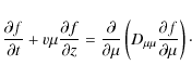
|
(59) |
To proceed, we compute the spatial average
|
(60) |
and the Fokker-Planck equation becomes
|
(61) |
By assuming that
![\begin{displaymath}{\partial F \over \partial t} = D {\partial \over \partial \mu} \left[ (1-\mu^2){\partial F \over \partial \mu} \right]\cdot
\end{displaymath}](/articles/aa/full_html/2009/44/aa12755-09/img172.png)
|
(62) |
This equation can be solved analytically without further assumptions. E.g., Shalchi (2006) has demonstrated that the solution of this equation can be expressed by Legendre polynomials
|
(63) |
For sharp initial conditions (
|
(64) |
An interesting property is the anisotropy A (t) which can be defined as
|
(65) |
With
|
(66) |
we find
In the last step we have used Eq. (1) for the parallel mean free path. Analytical results such as Eq. (67) can be compared with measurements of solar particle events by spacecrafts such as Wind (see, e.g., Dröge & Kartavykh 2009).
8.2 Interstellar propagation and steep spectra
![\begin{figure}
\par\includegraphics[width=8.8cm,clip]{12755fg6.eps}
\vspace*{3mm}
\end{figure}](/articles/aa/full_html/2009/44/aa12755-09/img182.png)
|
Figure 6:
|
| Open with DEXTER | |
In Lazar et al. (2003) and Spanier & Schlickeiser (2005),
the heating rate of the interstellar medium (ISM), especially the
warm ionized medium, has been calculated. Within these two papers it
was demonstrated that a steeper form of the turbulence spectrum (s > 2) could be reasonable. In this case we obtain
by employing standard QLT an infinitely large parallel mean free path (
![]() ). In Shalchi (2007) it has already been demonstrated the SOQLT is in agreement with simulations for such spectra.
In the present section we compare our analytical finding with these previous results (see Fig. 6).
). In Shalchi (2007) it has already been demonstrated the SOQLT is in agreement with simulations for such spectra.
In the present section we compare our analytical finding with these previous results (see Fig. 6).
For the analytical results we can use Eq. (51)
since we assume not too strong stochastic fields. These analytical
forms are only valid for smaller rigidities. For high particle energies
the analytical results
deviate from the numerical finding. For weak turbulence and s>2 we can derive from Eq. (51) the formula
| (68) |
For strong turbulence we have to use Eq. (49). The pitch-angle Fokker-Planck coefficient for high particle rigidities can be derived from Eq. (40). In this case it is also straightforward to compute the parallel mean free path.
8.3 The Hillas limit and high energetic cosmic rays
In Shalchi et al. (2009a)
we have investigated for the first time the propagation of ultrahigh
energy particles within the framework of SOQLT. In this article we have
computed numerically the
pitch-angle Fokker-Planck coefficient and the parallel mean free path.
As shown there, the Hillas
limit![]() is questionable.
is questionable.
It is the purpose of the present section to calculate analytically the
pitch-angle Fokker-Planck coefficient of very high energetic particles.
For simplicity we assume
![]() and we can use Eq. (33). By using a spectrum with sharp cutoff at short wavenumbers we find
and we can use Eq. (33). By using a spectrum with sharp cutoff at short wavenumbers we find
|
(69) |
To evaluate this formula we assume

|
(70) |
with the largest scale of the turbulence
![$\displaystyle D = \pi \Omega D(s, q) l_{\rm slab} \frac{\delta B^2}{B_0^2} \Gam...
... slab})^{q}}{\left[ 1 + (k_{\parallel} l_{\rm slab} )^2 \right]^{(s+q)/2}}\cdot$](/articles/aa/full_html/2009/44/aa12755-09/img191.png)
|
(71) |
With the integral transformation
|
(72) |
with
![\begin{displaymath}Q (s,q,x_{\min}) = \int_{x_{\min}}^{\infty} {\rm d} x \; \frac{x^{q-1}}{\left[ 1 + x^2 \right]^{(s+q)/2}}\cdot
\end{displaymath}](/articles/aa/full_html/2009/44/aa12755-09/img194.png)
|
(73) |
By using Gradshteyn & Ryzhik (2000) we can solve the integral to find
|
(74) |
Finally, we find for the pitch-angle Fokker-Planck coefficient of ultrahigh energetic particles
|
(75) |
By using Eq. (1) it is a simple matter to calculate analytically the parallel mean free path
This result is valid for
Quasilinear theory predicts that the parallel mean free path of particles with
![]() is infinity. Consequently, the motion of high energy particle is scatter-free (ballistic) and, therefore, such particles
cannot be confined to the Galaxy. According to Eq. (76),
however, we find finite scattering within the framework of SOQLT.
Therefore, we expect a finite confinement time of real particles in the
Galaxy. For details we refer to Shalchi et al. (2009).
is infinity. Consequently, the motion of high energy particle is scatter-free (ballistic) and, therefore, such particles
cannot be confined to the Galaxy. According to Eq. (76),
however, we find finite scattering within the framework of SOQLT.
Therefore, we expect a finite confinement time of real particles in the
Galaxy. For details we refer to Shalchi et al. (2009).
9 Summary and conclusion
In the present article we have revisited the problem of pitch-angle
scattering and parallel diffusion of
charged particles. Previous investigations are based on the quasilinear
approximation or on nonlinear
theories. In the latter case only numerical results were available for
the pitch-angle Fokker-Planck coefficient and the parallel mean free
path. In Sect. 3 we have explored for the first time analytically
the second order theory of Shalchi (2005a). By deriving general analytical expressions for the
parameter
![]() ,
we have shown that the traditional quasilinear theory is correct for
,
we have shown that the traditional quasilinear theory is correct for
![]() /B0 and the assumption of isotropic scattering
/B0 and the assumption of isotropic scattering
![]() is
valid for strong turbulence. This result confirms previous articles
about diffusive shock acceleration (see, e.g., Kirk & Schneider 1988; Schneider & Kirk 1989; Kirk & Schneider 1989). It should be noted, however, that for extremely strong turbulence one expects Bohm-diffusion (see Shalchi 2009a).
is
valid for strong turbulence. This result confirms previous articles
about diffusive shock acceleration (see, e.g., Kirk & Schneider 1988; Schneider & Kirk 1989; Kirk & Schneider 1989). It should be noted, however, that for extremely strong turbulence one expects Bohm-diffusion (see Shalchi 2009a).
By employing the spectrum of Shalchi & Weinhorst (2009a) we derived analytical forms for the Fokker-Planck
coefficient
![]() and the parallel mean free path
and the parallel mean free path
![]() .
The formulae for the
latter parameter can also be used for strong turbulence and for steep spectra (
.
The formulae for the
latter parameter can also be used for strong turbulence and for steep spectra (![]() ). Quasilinear
theory for parallel spatial diffusion is only valid for weak turbulence (
). Quasilinear
theory for parallel spatial diffusion is only valid for weak turbulence (
![]() )
and flat spectra
(s
< 2). For these spectra we have also introduced plasma wave
propagation effects by following Schlickeiser (2002). For particle
velocities satisfying
)
and flat spectra
(s
< 2). For these spectra we have also introduced plasma wave
propagation effects by following Schlickeiser (2002). For particle
velocities satisfying
![]() the quasilinear results obtained for the plasma wave model are correct since nonlinear effect are supressed. For
the quasilinear results obtained for the plasma wave model are correct since nonlinear effect are supressed. For
![]() nonlinear effects are stronger and the magnetostatic model should provide a good approximation.
nonlinear effects are stronger and the magnetostatic model should provide a good approximation.
Analytical forms for the parameters
![]() and
and
![]() are very useful in the physics of cosmic rays. Therefore, we have
presented some applications of our results (see Sect. 8). We have
shown how energetic particles from the Sun can be described
analytically be computing the anisotropy A. Such results can be compared with spacecraft observations such as Wind measurements (see, e.g.,
Dröge & Kartavykh 2009).
As a second example we computed the parallel mean free path of
particles in the ISM by assuming steep turbulence spectra as suggested
by Lazar et al. (2003) and Spanier & Schlickeiser
(2005). These analytical results complement the numerical work of Shalchi (2007). Standard quasilinear theory results in
are very useful in the physics of cosmic rays. Therefore, we have
presented some applications of our results (see Sect. 8). We have
shown how energetic particles from the Sun can be described
analytically be computing the anisotropy A. Such results can be compared with spacecraft observations such as Wind measurements (see, e.g.,
Dröge & Kartavykh 2009).
As a second example we computed the parallel mean free path of
particles in the ISM by assuming steep turbulence spectra as suggested
by Lazar et al. (2003) and Spanier & Schlickeiser
(2005). These analytical results complement the numerical work of Shalchi (2007). Standard quasilinear theory results in
![]() for such spectra. We have also considered the problem of ultrahigh
energy cosmic rays. These results complement the numerical work of
Shalchi et al. (2009a). We have derived for the first time a formula for the parallel mean free path of ultrahigh energy cosmic rays
within SOQLT. According to this formula we have
for such spectra. We have also considered the problem of ultrahigh
energy cosmic rays. These results complement the numerical work of
Shalchi et al. (2009a). We have derived for the first time a formula for the parallel mean free path of ultrahigh energy cosmic rays
within SOQLT. According to this formula we have
![]() /
/![]() if the particle Larmor radius exceeds the largest scale of turbulence (
if the particle Larmor radius exceeds the largest scale of turbulence (
![]() ). We expect that our analytical results will lead to further interesting and important applications in astrophysics such as
diffusive shock acceleration.
). We expect that our analytical results will lead to further interesting and important applications in astrophysics such as
diffusive shock acceleration.
This research was supported by the Deutsche Forschungsgemeinschaft (DFG) under the Emmy-Noether Programm (grant SH 93/3-1) and project Schl 201/19-1. As a member of the Junges Kolleg, A. Shalchi also acknowledges support by the Nordrhein-Westfälische Akademie der Wissenschaften.
References
- Abramowitz, M., & Stegun, I. A. 1974, Handbook of Mathematical Functions (New York: Dover Publications)
- Alania, M. V., & Wawrzynczak, A. 2008, Astrophys. Space Sci. Trans., 4, 59 [NASA ADS]
- Dröge, W. 2000, Space Sci. Rev., 93, 121 [CrossRef] [NASA ADS]
- Dröge, W., & Kartavykh, Y. Y. 2009, ApJ, 693, 69 [CrossRef] [NASA ADS]
- Earl, J. A. 1974, ApJ, 193, 231 [CrossRef] [NASA ADS]
- Fletcher, L. 1997, A&A, 326, 1259 [NASA ADS]
- Giacalone, J., & Jokipii, J. R. 1999, ApJ, 520, 204 [CrossRef] [NASA ADS]
- Gkioulidou, M., Zimbardo, G., Pommois, P., Veltri, P., & Vlahos, L. 2007, A&A, 462, 1113 [EDP Sciences] [CrossRef] [NASA ADS]
- Goldstein, M. L. 1976, ApJ, 204, 900 [CrossRef] [NASA ADS]
- Gradshteyn, I. S., & Ryzhik, I. M. 2000, Table of integrals, series, and products (New York: Academic Press)
- Green, M. S. 1951, J. Chem. Phys., 19, 1036 [CrossRef] [NASA ADS]
- Hillas, A. M. 1984, ARA&A, 22, 425 [CrossRef] [NASA ADS]
- Jokipii, J. R. 1966, ApJ, 146, 480 [CrossRef] [NASA ADS]
- Jones, F. C., Kaiser, T. B., & Birmingham, T. J. 1973, PRL, 31, 485 [CrossRef] [NASA ADS]
- Jones, F. C., Birmingham, T. J., & Kaiser, T. B. 1978, Phys. Fluids, 21, 347 [CrossRef] [NASA ADS]
- Kubo, R. 1957, J. Phys. Soc. Jpn., 12, 570 [CrossRef] [NASA ADS]
- Kirk, J. G., & Schneider, P. 1988, A&A, 201, 177 [NASA ADS]
- Kirk, J. G., & Schneider, P. 1989, A&A, 225, 559 [NASA ADS]
- Lazar, M., Spanier, F., & Schlickeiser, R. 2003, A&A, 410, 415 [EDP Sciences] [CrossRef] [NASA ADS]
- Li, G., Zank, G. P., & Rice, W. K. M. 2003, J. Geophys. Res., 108, 1082 [CrossRef]
- Li, G., Zank, G. P., & Rice, W. K. M. 2005, J. Geophys. Res., 110, A06104 [CrossRef]
- Owens, A. J. 1974, ApJ, 191, 235 [CrossRef] [NASA ADS]
- Schlickeiser, R. 1989, ApJ, 336, 243 [CrossRef] [NASA ADS]
- Schlickeiser, R. 2002, Cosmic Ray Astrophysics (Berlin, Heidelberg: Springer-Verlag)
- Schneider, P., & Kirk, J. G. 1989, A&A, 217, 344 [NASA ADS]
- Shalchi, A. 2005, Phys. Plasmas, 12, 052324 [CrossRef]
- Shalchi, A. 2006, A&A, 448, 809 [EDP Sciences] [CrossRef] [NASA ADS]
- Shalchi, A. 2007, J. Phys. G., 34, 209 [CrossRef] [NASA ADS]
- Shalchi, A. 2009a, Astropart. Phys., 31, 237 [CrossRef] [NASA ADS]
- Shalchi, A. 2009b, Nonlinear Cosmic Ray Diffusion Theories, Astrophysics and Space Science Library, 362 (Berlin: Springer)
- Shalchi, A., & Schlickeiser, R. 2005, ApJ, 626, L97 [CrossRef] [NASA ADS]
- Shalchi, A., & Dosch, A. 2009, PRD, 79, 083001 [CrossRef] [NASA ADS]
- Shalchi, A., & Weinhorst, B. 2009, Adv. Space Res., 43, 1429 [CrossRef] [NASA ADS]
- Shalchi, A., Bieber, J. W., Matthaeus, W. H., & Schlickeiser, R. 2006, ApJ, 642, 2 [CrossRef]
- Shalchi, A., Skoda, T., Tautz, R. C., & Schlickeiser, R. 2009, PRD, 80, 023012 [CrossRef] [NASA ADS]
- Spanier, F., & Schlickeiser, R. 2005, A&A, 436, 9 [EDP Sciences] [CrossRef] [NASA ADS]
- Tautz, R. C., Shalchi, A., & Schlickeiser, R. 2008, ApJ, 685, L165 [CrossRef] [NASA ADS]
- Taylor, G. I. 1922, Diffusion by continuous movement, Proceedings of the London Mathematical Society, 20, 196
- Teufel, A., & Schlickeiser, R. 2002, A&A, 393, 703 [EDP Sciences] [CrossRef] [NASA ADS]
- Teufel, A., & Schlickeiser, R. 2003, A&A, 397, 15 [EDP Sciences] [CrossRef] [NASA ADS]
- Völk, H. J. 1973, Ap&SS, 25, 471 [CrossRef] [NASA ADS]
- Völk, H. J. 1975, Rev. Geophys. Space Phys., 13, 547 [CrossRef] [NASA ADS]
- Yan, H., & Lazarian, A. 2002, PRL, 89, 281102 [CrossRef] [NASA ADS]
- Zank, G. P., Rice, W. K. M., & Wu, C. C. 2000, J. Geophys. Res., 105, 25079 [CrossRef] [NASA ADS]
- Zank, G. P., Li, G., Florinski, V., et al. 2006, J. Geophys. Res., 111, A06108 [CrossRef]
Footnotes
- ... fields
![[*]](/icons/foot_motif.png)
- In the current article we neglect electric fields since they are less important for spatial diffusion. If one is interested in stochastic acceleration, however, electric fields are relevant (see, e.g., Schlickeiser 2002).
- ...2005)
- The resonance function of Eq. (9) was obtained by Shalchi (2005) by combining a second order approach
in combination with two mathematical approximations, namely a Late-Time-Approximation (LTA) and a
 -approximation. These approximations were employed to ensure mathematical tractability. For a
detailed explanation of these approximations and their justifications we refer to Shalchi (2005, 2009b).
-approximation. These approximations were employed to ensure mathematical tractability. For a
detailed explanation of these approximations and their justifications we refer to Shalchi (2005, 2009b).
- ... turbulence
- The bendover or turnover scale denotes the frequency break between the large scales (energy range) and the intermediate scales (inertial range) of the turbulence. For the spectrum defined in Eq. (34) the bendover scale is directly proportional to the turbulence correlation length.
- ...
limit
- Within the framework of magnetostatic quasilinear theory, the
resonance function is a sharp delta function. Since there exists a
largest scale of turbulence
 ,
ultrahigh energy particles having a Larmor radius larger than this scale (
,
ultrahigh energy particles having a Larmor radius larger than this scale (
 )
cannot be scattered and, therefore, they cannot be confined to the Galaxy. This limit is known as the Hillas limit (Hillas 1984).
)
cannot be scattered and, therefore, they cannot be confined to the Galaxy. This limit is known as the Hillas limit (Hillas 1984).
All Tables
Table 1: Parameters used in the present article.
Table 2: Plasmawave propagation versus nonlinearity.
All Figures
|
|
Figure 1: The particle motion through the turbulent plasma. The turbulent magnetic field is represented by the dashed line. If there would be no interaction between the plasma and the cosmic rays, the particles would follow unperturbed orbits (dotted line). The latter trajectories are used in quasilinear theory. In reality, however, the particles experience scattering and, therefore, the true orbits decorrelate from the unperturbed motion (solid lines). |
| Open with DEXTER | |
| In the text | |
|
|
Figure 2:
The different resonance functions
|
| Open with DEXTER | |
| In the text | |
|
|
Figure 3:
Shown are the results of QLT (dotted line), SOQLT within the |
| Open with DEXTER | |
| In the text | |
|
|
Figure 4: Enlarge of Fig. 3 at small pitch-angle cosines. |
| Open with DEXTER | |
| In the text | |
|
|
Figure 5: The parallel mean free path computed by using QLT (dotted line) for s=5/3. Also shown are the analytical results of SOQLT, namely the weak turbulence solution (dashed line) of Eq. (51) and the strong turbulence solution (solid line) of Eq. (49). |
| Open with DEXTER | |
| In the text | |
|
|
Figure 6:
|
| Open with DEXTER | |
| In the text | |
Copyright ESO 2009
Current usage metrics show cumulative count of Article Views (full-text article views including HTML views, PDF and ePub downloads, according to the available data) and Abstracts Views on Vision4Press platform.
Data correspond to usage on the plateform after 2015. The current usage metrics is available 48-96 hours after online publication and is updated daily on week days.
Initial download of the metrics may take a while.