| Issue |
A&A
Volume 503, Number 1, August III 2009
|
|
|---|---|---|
| Page(s) | 25 - 34 | |
| Section | Cosmology (including clusters of galaxies) | |
| DOI | https://doi.org/10.1051/0004-6361/200912234 | |
| Published online | 02 July 2009 | |
The onset of star formation in primordial haloes
U. Maio1,2 - B. Ciardi1 - N. Yoshida3 - K. Dolag1 - L. Tornatore4
1 - Max-Planck-Institut fuer Astrophysik,
Karl-Schwarzschild-Straße 1, 85748 Garching bei München, Germany
2 -
Max-Planck-Institut fuer extraterrestrische physik,
Giessenbachstraße 1, 85748 Garching bei München, Germany
3 -
IPMU, U-Tokyo
5-1-5 Kashiwanoha, Kashiwa, Chiba 277-8568, Japan
4 -
INAF - Osservatorio astronomico di Trieste,
via Tiepolo 11, 34143 Trieste, Italy
Received 30 March 2009 / Accepted 26 May 2009
Abstract
Context. Star formation remains an unsolved problem in astrophysics. Numerical studies of large-scale structure simulations cannot resolve the process and their approach usually assumes that only gas denser than a typical threshold can host and form stars.
Aims. We investigate the onset of cosmological star formation and compare several very-high-resolution, three-dimensional, N-body/SPH simulations that include non-equilibrium, atomic and molecular chemistry, star formation prescriptions, and feedback effects.
Methods. We study how primordial star formation depends on gas density threshold, cosmological parameters, and initial set-ups.
Results. For mean-density initial conditions, we find that standard low-density star-formation threshold (
![]() )
models predict the onset of star formation at
)
models predict the onset of star formation at ![]() -31, depending on the adopted cosmology. In these models, stars are formed automatically when the gas density increases above the adopted threshold, regardless of the time between the moment when the threshold is reached and the effective runaway collapse. While this is a reasonable approximation at low redshift, at high redshift this time interval represents a significant fraction of the Hubble time and thus this assumption can induce large artificial offsets to the onset of star formation. Choosing higher density thresholds (
-31, depending on the adopted cosmology. In these models, stars are formed automatically when the gas density increases above the adopted threshold, regardless of the time between the moment when the threshold is reached and the effective runaway collapse. While this is a reasonable approximation at low redshift, at high redshift this time interval represents a significant fraction of the Hubble time and thus this assumption can induce large artificial offsets to the onset of star formation. Choosing higher density thresholds (
![]() )
allows the entire cooling process to be followed, and the onset of star formation is then estimated to be at redshift
)
allows the entire cooling process to be followed, and the onset of star formation is then estimated to be at redshift ![]() -16. When isolated, rare, high-density peaks are considered, the chemical evolution is much faster and the first star formation episodes occur at
-16. When isolated, rare, high-density peaks are considered, the chemical evolution is much faster and the first star formation episodes occur at
![]() ,
almost regardless of the choice of the density threshold.
,
almost regardless of the choice of the density threshold.
Conclusions. These results could have implications for the formation redshift of the first cosmological objects, as inferred from direct numerical simulations of mean-density environments and studies of the reionization history of the universe.
Key words: methods: N-body simulations - large-scale structure of Universe - early Universe
1 Introduction
Understanding primordial structure formation is one of the fundamental
issues of modern astrophysics and cosmology. There is wide
agreement that not only consists the universe of ordinary ``baryonic''
matter but also a large fraction of unknown ``dark'' matter, whose effects
are only gravitational.
Baryonic matter appears to
constitute only a small fraction of the total cosmological matter
content with a present-day density parameter
![]() compared to
compared to
![]() (Hinshaw et al. 2008).
Since the universe is observed to have zero curvature, i.e. to have a
total density parameter
(Hinshaw et al. 2008).
Since the universe is observed to have zero curvature, i.e. to have a
total density parameter
![]() ,
these
data imply that an additional density term exists
,
these
data imply that an additional density term exists
![]() .
This is probably related to the so-called ``cosmological constant''
(Einstein 1917), or, as initially suggested by
Ratra & Peebles (1988), Wetterich (1988), Brax & Martin (1999) and Peebles & Ratra (2003),
to other kinds of unknown ``dark energies'', whose effects on early
structure formation history have been studied by e.g.
Maio et al. (2006) with numerical simulations and by
Crociani et al. (2008) with analytical calculations.
.
This is probably related to the so-called ``cosmological constant''
(Einstein 1917), or, as initially suggested by
Ratra & Peebles (1988), Wetterich (1988), Brax & Martin (1999) and Peebles & Ratra (2003),
to other kinds of unknown ``dark energies'', whose effects on early
structure formation history have been studied by e.g.
Maio et al. (2006) with numerical simulations and by
Crociani et al. (2008) with analytical calculations.
The existence of non-baryonic matter was suggested several decades ago, and structure formation models based on the growth of primordial gravitational instabilities (White & Rees 1978; Peebles 1974) were developed following the early work by Gunn & Gott (1972).
Hydrodynamical simulation codes (the first dating back to Evrard 1988; and Hernquist & Katz 1989) have become a powerful tool, but because of computational limitations, plausible subgrid models have always been required to take into account star formation events (e.g. Schaye & Dalla Vecchia 2008; Springel & Hernquist 2003; Cen & Ostriker 1992; Katz et al. 1996; Dalla Vecchia & Schaye 2008; Katz 1992). These simulations model the converging gas infall into dark-matter potential wells, by following the gas that becomes shock heated and subsequently cools by atomic and/or molecular cooling. Given the many orders of magnitude (in scale and density) spanned, it is computationally extremely challenging to simulate the process down to the formation of single stars.
The gas physics in structure formation simulations has been typically approached with either lagrangian smoothed particle hydro-dynamics (SPH) or Eulerian mesh codes. A particular subclass is constituted by adaptive mesh refinement (AMR) codes, which allow further decomposition of the mesh around high-density regions, achieving a higher resolution. The main advantage of the SPH approach is its ability to follow self gravity in detail, while hydrodynamical instabilities are usually captured by mesh codes.
To account for star-formation episodes, both SPH and mesh schemes rely on specific assumptions. The prescriptions applied in mesh codes (e.g. Cen & Ostriker 1992; Inutsuka & Miyama 1992; Truelove et al. 1997) usually assume that the star formation rate is proportional to the density of overdense gas, while those used in SPH codes (e.g. Springel & Hernquist 2003; Bate & Burkert 1997; Katz 1992) are based on the existence of a density threshold above which the gas is gradually converted into stars. Here we make use of SPH simulations.
The typical timescales involved in the process of gas condensation
are the free-fall time,
![]() ,
and the cooling time,
,
and the cooling time,
![]() .
Gas condensation is expected to take place only if
.
Gas condensation is expected to take place only if
![]() .
.
The free-fall time is defined as

where G is the universal gravitational constant and

where n is the number density of the gas,
with the quantum-mechanical function
The physical conditions in which the first structures form are characterized by a primordial chemical composition: mostly hydrogen, deuterium, helium, and some simple molecules, e.g. H2 and HD.
The primordial sites in which the first stars form are thought to be
small dark-matter haloes with masses ![]()
![]() - as
expected from predictions based on self-similar gravitational
condensation and chemical evolution
(e.g. Trenti & Stiavelli 2009; Tegmark et al. 1997)
- and virial temperatures
- as
expected from predictions based on self-similar gravitational
condensation and chemical evolution
(e.g. Trenti & Stiavelli 2009; Tegmark et al. 1997)
- and virial temperatures
![]() K.
Once they are born, they illuminate the universe and mark the end of
the ``dark ages''.
The radiation propagates in the vicinity of the individual sources and
the impact on the subsequent structure formation (Ricotti et al. 2002b,a,2008) can be very
significant leaving imprints by a means of feedback effects
(see Ciardi & Ferrara 2005, for a review).
K.
Once they are born, they illuminate the universe and mark the end of
the ``dark ages''.
The radiation propagates in the vicinity of the individual sources and
the impact on the subsequent structure formation (Ricotti et al. 2002b,a,2008) can be very
significant leaving imprints by a means of feedback effects
(see Ciardi & Ferrara 2005, for a review).
The low virialization temperatures of primordial
haloes are enough neither to excite nor to ionize hydrogen and
the lack of any metals means that the gas can cool and eventually
form objects only via molecular transitions (Hollenbach & McKee 1979; Peebles & Dicke 1968; Saslaw & Zipoy 1967, Maio et al. 2007, for a detailed
study of the cooling efficiency in different
regimes).
They have rotational energy separations
with excitation temperatures below 104 K, and therefore it is
possible to collisionally populate their higher levels with the consequent
emission of radiation and resulting gas cooling. Since the
molecular energy-state separations are typically smaller than the
atomic ones, cooling will of course be slower, but still capable of bringing
the temperature down to ![]() 102 K
(Yoshida et al. 2006,2003; Gao et al. 2007; Omukai & Palla 2003).
102 K
(Yoshida et al. 2006,2003; Gao et al. 2007; Omukai & Palla 2003).
To follow the entire process of structure and star formation in numerical simulations, one should implement the entire set of chemical reactions and hydrodynamical equations and from those calculate the abundance evolution and the corresponding cooling terms. In practice, performing these computations is very expensive and time consuming and it becomes extremely challenging to follow the formation of structures from the initial gas infall into the dark-matter potential wells to the final birth of stars. Nevertheless, efforts are being made in this direction (e.g. Whalen et al. 2008; Bromm & Larson 2004; Abel et al. 2002; Yoshida et al. 2007).
For this reason, more practical, even if sometimes
coarse, simple models are adopted.
In brief, star formation relies on semi-empirical and numerical
recipes based on chosen criteria to convert gas into stars and obtain
the star formation rate, carefully normalized to fit observational
data at the present day.
In particular, in SPH approaches a single particle represents a
population of stars with assigned mass distribution.
The standard method used is to assume that once the gas has
reached a given density threshold it automatically forms
stars![]() (e.g Cen & Ostriker 1992; Katz 1992; Katz et al. 1996, and the popular Springel & Hernquist 2003, model, inspired by the previous works),
regardless of the time between the moment when the threshold is
reached and the effective run-away collapse, which typically takes
place at densities
(e.g Cen & Ostriker 1992; Katz 1992; Katz et al. 1996, and the popular Springel & Hernquist 2003, model, inspired by the previous works),
regardless of the time between the moment when the threshold is
reached and the effective run-away collapse, which typically takes
place at densities ![]() 102-
102-
![]() .
While this is a reasonable approximation at low redshift, in ``average''
regions of the universe at
high redshift this time interval represents a significant fraction of the
Hubble time and thus the assumption can induce large artificial
offsets on the onset of star formation and influence the evolution in
the derived star formation rate.
Thus, extrapolations to high redshifts of the low-density thresholds
(few
.
While this is a reasonable approximation at low redshift, in ``average''
regions of the universe at
high redshift this time interval represents a significant fraction of the
Hubble time and thus the assumption can induce large artificial
offsets on the onset of star formation and influence the evolution in
the derived star formation rate.
Thus, extrapolations to high redshifts of the low-density thresholds
(few
![]() )
used to model the star formation rate in the
low-redshift universe, may not always be justifiable.
For this reason, high-redshift applications require higher resolutions
and a higher density threshold.
)
used to model the star formation rate in the
low-redshift universe, may not always be justifiable.
For this reason, high-redshift applications require higher resolutions
and a higher density threshold.
In this paper, we are interested in modeling star formation as a global process in regions of mean density in the universe, not directly in the very first stars, which instead form in highly overdense, isolated regions. In particular, we discuss the importance of the choice of the density threshold for star formation in simulations of early structure formation. We present a criterion to choose this threshold (Sect. 2) and some test cases based on high-resolution simulations (Sects. 3 and 4). Then we present our results and conclusions (Sect. 5).
2 Threshold for star formation
According to the usual scenario of structure formation, the Jeans
mass (Jeans 1902) is the fundamental quantity that allows us to
distinguish collapsing from non-collapsing objects, under gravitational
instability.
For a perfect, isothermal gas, it is given by
 |
(4) |
where
As mentioned in the introduction, the density threshold for star formation in numerical simulations is typically fixed to some constant value, irrespective of the simulation resolution. However, it would be desirable to have a star formation criterion that allows us to reach scales that fully resolve the Jeans mass.
The SPH algorithm implicitly imposes a minimum mass resolution limit,
because to compute the different physical
quantities, a fixed number of neighbours (i.e. number of particles
within the smoothing length![]() , h) is used.
This also induces a minimum resolvable mass, which is the total mass of
neighbouring particles.
This is particularly important in SPH simulations of
cosmological structures and galaxy formation, because only
if the minimum resolvable mass is far smaller than the Jeans mass, it
is possible to ensure that the results are not affected by numerics
nor by the details of the implementation adopted
(Bate & Burkert 1997).
Otherwise, unresolved, Jeans unstable clumps can easily be found to exhibit
unphysical behaviour (e.g. over-fragmentation problem in low-resolution simulations). Furthermore, it was shown
(Bate & Burkert 1997; Navarro & White 1993) that the minimum
number of particles needed to obtain reasonable and converging results
is about twice the number of neighbours (
, h) is used.
This also induces a minimum resolvable mass, which is the total mass of
neighbouring particles.
This is particularly important in SPH simulations of
cosmological structures and galaxy formation, because only
if the minimum resolvable mass is far smaller than the Jeans mass, it
is possible to ensure that the results are not affected by numerics
nor by the details of the implementation adopted
(Bate & Burkert 1997).
Otherwise, unresolved, Jeans unstable clumps can easily be found to exhibit
unphysical behaviour (e.g. over-fragmentation problem in low-resolution simulations). Furthermore, it was shown
(Bate & Burkert 1997; Navarro & White 1993) that the minimum
number of particles needed to obtain reasonable and converging results
is about twice the number of neighbours (![]() 102 particles).
102 particles).
If
![]() is the gas mass resolution of a given
simulation, we can assume that:
is the gas mass resolution of a given
simulation, we can assume that:
| (5) |
where
![$\displaystyle \frac{1.31\times 10^{-13}}{N^2} \left(
\frac{M_{\rm res}}{ M_{\od...
...3~{\rm K}}\right)^{\!3} \!\!\left( \frac{1}{\mu}\right)^{\!3}~~\rm [g~cm^{-3}].$](/articles/aa/full_html/2009/31/aa12234-09/img54.png)
For
In general, in simulations of both cosmic structure and galaxy formation, it is quite hard to fully resolve the Jeans mass of the collapsing fragments, and star formation is often assumed to occur while the gas falling into the dark-matter potential wells is still heating up. The Bate & Burkert (1997) requirement is not usually satisfied, since the main goal is usually not to follow the entire process of collapse and fragmentation, but to obtain a qualitatively representative sample of the cosmological evolution.
A high value for the threshold is also important to capture the relevant
phases of cooling.
In the following, we show that molecule radiative losses, at
temperatures of ![]()
![]() where they can balance the
heating of the infalling gas, produce an isothermal state and a
subsequent cooling regime.
For a region of mean density, the time spent by the gas in the
isothermal state can be a substantial fraction of the Hubble time.
Therefore, it is important for the threshold to be
on the right-hand side of the peak in the phase-diagram (i.e. at densities
higher than the isothermal regime), so that the delay between reaching the
threshold and the true star formation is negligible (see Sect. 4).
where they can balance the
heating of the infalling gas, produce an isothermal state and a
subsequent cooling regime.
For a region of mean density, the time spent by the gas in the
isothermal state can be a substantial fraction of the Hubble time.
Therefore, it is important for the threshold to be
on the right-hand side of the peak in the phase-diagram (i.e. at densities
higher than the isothermal regime), so that the delay between reaching the
threshold and the true star formation is negligible (see Sect. 4).
In the following, we investigate the effect of different choices of star formation thresholds at high redshift, describe the simulations performed, and discuss the results obtained.
Table 1: Parameters adopted for the simulations.
3 Simulation set-up
To study the effect of different threshold prescriptions on the onset of star formation, we completed very high resolution, three-dimensional, hydrodynamic simulations including non-equilibrium atomic and molecular chemistry, star formation, and wind feedback.
We used the code Gadget-2 (Springel 2005)
in its modified form, which includes stellar evolution and metal
pollution (Tornatore et al. 2007a), primordial molecular chemistry (following
the evolution of e-, H, H+, He, He+, He++, H2,
H+2, H-, D, D+, HD, ![]() ), and fine structure metal
transition cooling (O, C+, Si+, Fe+) at temperatures lower
than 104 K (Maio et al. 2007,2008).
We perform hydro-calculations by fixing the number of SPH neighbours to
), and fine structure metal
transition cooling (O, C+, Si+, Fe+) at temperatures lower
than 104 K (Maio et al. 2007,2008).
We perform hydro-calculations by fixing the number of SPH neighbours to
![]() .
.
The simulations have a comoving box size of
![]() and sample the cosmological medium with a uniform realization of
3203 particles for both gas and dark-matter species (for a total
number of
and sample the cosmological medium with a uniform realization of
3203 particles for both gas and dark-matter species (for a total
number of
![]() particles).
The resulting gas-particle mass is of the order of
particles).
The resulting gas-particle mass is of the order of
![]() ,
which is consistent with the discussion in the previous section.
,
which is consistent with the discussion in the previous section.
We note that this configuration enables us to easily resolve the Jeans
length for shock heated/cooling cosmic gas (the Jeans length for
gas with
![]() and
and
![]() -
-
![]() is
is ![]() 3-
3-
![]() ,
much longer than the comoving gravitational softening
,
much longer than the comoving gravitational softening![]() of
of ![]()
![]() ).
).
The initial conditions (set at redshift z=100) are
generated with a fast Fourier transform grid of
![]() meshes and a maximum wave-number (Nyquist frequency)
meshes and a maximum wave-number (Nyquist frequency)
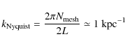 |
(i.e. a minimum wavelength of
We will refer to this sampling as ``mean region''.
We considered two different sets of cosmological parameters:
-
standard model:
 ,
,
 ,
,
 ,
h=0.7,
,
h=0.7,
 and n=1, where the
symbols have the usual meanings.
The corresponding dark-matter and gas-particle masses are
and n=1, where the
symbols have the usual meanings.
The corresponding dark-matter and gas-particle masses are 
 and
and
 ,
respectively.
,
respectively.
-
WMAP5 model: data from 5-year WMAP (WMAP5) satellite
(Hinshaw et al. 2008) suggest that
 ,
,
 ,
,
 ,
h=0.72,
,
h=0.72,
 ,
and
n=0.96.
In this case, the corresponding
dark-matter and gas-particle masses are
,
and
n=0.96.
In this case, the corresponding
dark-matter and gas-particle masses are
 and
and
 ,
respectively.
,
respectively.
Following the discussion in the previous sections, we also consider two different values for the star formation density threshold:
-
a low-density threshold of
 (physical), compatible with the one adopted in the Gadget code and the
ones widely used in the literature (for example Springel & Hernquist 2003; Tornatore et al. 2007b; Pawlik et al. 2009; Katz et al. 1996);
(physical), compatible with the one adopted in the Gadget code and the
ones widely used in the literature (for example Springel & Hernquist 2003; Tornatore et al. 2007b; Pawlik et al. 2009; Katz et al. 1996);
-
a high-density threshold of
 (physical),
as computed from Eqs. (6) and (7). This
value is adequate for modelling atomic processes even in small
(physical),
as computed from Eqs. (6) and (7). This
value is adequate for modelling atomic processes even in small
 haloes at
  .
Moreover, this threshold typically falls in density regimes where
cooling dominates over heating, allowing us to properly resolve
gas condensation down to the bottom of the cooling branch.
.
Moreover, this threshold typically falls in density regimes where
cooling dominates over heating, allowing us to properly resolve
gas condensation down to the bottom of the cooling branch.
A summary of all the simulation features is given in Table 1. We denote with the labels ``std'' and ``wmap5'' the runs with standard and WMAP5 cosmology, respectively, and with ``lt'' and ``ht'' the runs with low- and high-density thresholds, respectively.
We note that the Springel & Hernquist (2003) model used here to describe the star formation process is strictly applicable only as long as more than one star per SPH particle is present, i.e. each SPH particle is considered as a ``simple stellar populationÃ'' with a given mass distribution. Although some studies (Bromm & Larson 2004; Yoshida et al. 2003; Bromm et al. 2002) seem to indicate (or assume) that the very first episode of star formation could result in a single, very massive star per halo, this should apply preferentially to very high redshift, high density, isolated objects. In any case, the exact shape of the IMF of primordial stars (e.g. Schwarzschild & Spitzer 1953; Nakamura & Umemura 2001; Omukai & Palla 2003; Larson 1998) is still a matter of speculation and lively debate. For this reason and because we are interested mainly in the global star formation process, we used the Springel & Hernquist (2003) model (as Tornatore et al. 2007b, also did to describe both a primordial top-heavy and a more standard star formation mode) and allowed the IMF to be a free parameter (although in the test cases reported here we always adopt a top-heavy IMF). The aim of this paper is to investigate the effects of the density threshold on star formation, and we leave discussion on the IMF to future work.
Finally, to investigate primordial star formation events in
local high-density regions, we perform a very high-resolution numerical
simulation of a rare high-sigma peak with comoving radius ![]()
![]() .
This region is selected using the zoomed initial condition technique
on a
.
This region is selected using the zoomed initial condition technique
on a ![]()
![]() halo formed in a dark-matter-only
simulation (Gao et al. 2007)
halo formed in a dark-matter-only
simulation (Gao et al. 2007)![]() .
We divided each particle into gas and dark-matter component, according to
the standard model parameters.
The resulting gas-particle mass is
.
We divided each particle into gas and dark-matter component, according to
the standard model parameters.
The resulting gas-particle mass is ![]()
![]() and dark
matter particles have a mass of
and dark
matter particles have a mass of ![]()
![]() (in Table 1, this simulation is labelled ``zoom-std-ht'').
(in Table 1, this simulation is labelled ``zoom-std-ht'').
By a quick comparison of the different parameters adopted, we expect that, once the density threshold has been fixed, the standard cosmological mean-region simulations will show earlier structure formation episodes with respect to the corresponding wmap5 ones. This is because they have higher spectral parameters and higher matter content. The high-density region is a biased over-dense region already at early times, and therefore, its evolution is expected to be much faster.
4 Results
We present the results of the simulations with the sets of parameters described above. We discuss first the mean region of the universe (Sect. 4.1) and then the high-density region (Sect. 4.2).
![\begin{figure}
\par\begin{tabular}{ccc}
&\hspace{0.2\textwidth} {\bf Mean-region...
...phics[width=5.2cm]{figure/fig1bottom/19288_16.eps} }
\vspace{0.5cm}
\end{figure}](/articles/aa/full_html/2009/31/aa12234-09/img110.png) |
Figure 1:
First, second, and third column are respectively
temperature, density, and molecule maps.
The first two rows refer to the mean-region simulation at redshift
12.17 ( top) and 30.16 ( bottom).
The box size is 1 Mpc comoving.
The last two rows refer to the high-density region at redshift
50 ( top) and 70 ( bottom).
The region size is |
| Open with DEXTER | |
4.1 Mean-region simulation
Our reference run is the wmap5-ht model with initial composition given by the values quoted in Galli & Palla (1998)
![\begin{figure}
\par\includegraphics[width=9cm,clip]{19288_2.eps}
\end{figure}](/articles/aa/full_html/2009/31/aa12234-09/img120.png) |
Figure 2:
Upper panel:
phase diagram at redshift z=12.17 (just before the onset of
star formation) for the wmap5-ht simulation.
The vertical straight lines indicate a
low physical critical density threshold of
|
| Open with DEXTER | |
The solid vertical line corresponds to the physical high-density star
formation threshold (
![]() )
and, for comparison, we
also plot the dashed line for a physical number density of
)
and, for comparison, we
also plot the dashed line for a physical number density of
![]() .
We stress that by adopting a low-density threshold for star
formation one completely misses the isothermal and cooling part of
the phase diagram, and thus a correct modeling of the cooling
regions within the simulations. This can affect the onset of star
formation, particularly at high redshift, when the time needed for the gas
to evolve from the low-density threshold to the high-density threshold
(
.
We stress that by adopting a low-density threshold for star
formation one completely misses the isothermal and cooling part of
the phase diagram, and thus a correct modeling of the cooling
regions within the simulations. This can affect the onset of star
formation, particularly at high redshift, when the time needed for the gas
to evolve from the low-density threshold to the high-density threshold
(![]()
![]() )
can be a substantial fraction of
the Hubble time (
)
can be a substantial fraction of
the Hubble time (![]()
![]() at
at ![]() ). We note that
the time elapsed between the attainment of the isothermal peak in the
phase diagram and the end of the cooling branch is
). We note that
the time elapsed between the attainment of the isothermal peak in the
phase diagram and the end of the cooling branch is ![]()
![]() .
The evolution that follows the end of the cooling branch
is characterized by the formation of a dense core, which accretes gas
on free-fall timescales (Yoshida et al. 2006).
This phase has a very short duration (
.
The evolution that follows the end of the cooling branch
is characterized by the formation of a dense core, which accretes gas
on free-fall timescales (Yoshida et al. 2006).
This phase has a very short duration (![]() 106-
106-
![]() )
during which the
central densities increase to
)
during which the
central densities increase to ![]()
![]() .
The problem is less severe at lower redshift, when the Hubble time
becomes of the order of several Gyr.
.
The problem is less severe at lower redshift, when the Hubble time
becomes of the order of several Gyr.
![\begin{figure}
\par\includegraphics[width=9cm,clip]{19288_3.eps}
\end{figure}](/articles/aa/full_html/2009/31/aa12234-09/img126.png) |
Figure 3: Evolution of the ten most massive haloes in the wmap5-ht cosmological simulation (dotted lines). The redshift at which the first star forms in each halo is indicated by the filled star symbols. After that, star formation continues along the solid lines. |
| Open with DEXTER | |
The density and temperature behaviour can also be described
by an effective index![]() ,
which depends on the physical conditions of the gas regime
considered.
In the lower panel of Fig. 2, we plot the effective
index as a function of density.
The solid line refers to the value
,
which depends on the physical conditions of the gas regime
considered.
In the lower panel of Fig. 2, we plot the effective
index as a function of density.
The solid line refers to the value
![]() ,
which takes into account changes in the sign of the temperature
derivative, distinguishing the heating regime (
,
which takes into account changes in the sign of the temperature
derivative, distinguishing the heating regime (![]() )
from the
cooling regime (
)
from the
cooling regime (![]() )
.
The dashed line refers to
)
.
The dashed line refers to
![]() ,
so that
,
so that ![]() is always
is always ![]() 1.
Dotted horizontal straight lines INDICATE values of 5/3, 1, and
1/3.
In correspondence with the isothermal peak in the
1.
Dotted horizontal straight lines INDICATE values of 5/3, 1, and
1/3.
In correspondence with the isothermal peak in the ![]() plane,
it is
plane,
it is
![]() ,
which marks the transition from the heating
to the cooling regime.
At this stage, we expect the gas runaway collapse to begin and last
for the following cooling regime, at which point
,
which marks the transition from the heating
to the cooling regime.
At this stage, we expect the gas runaway collapse to begin and last
for the following cooling regime, at which point ![]() oscillates around the value of 1/3.
oscillates around the value of 1/3.
In Fig. 3, we plot the evolution of the ten most
massive haloes found in the simulation. We also show the redshift at which
stars are produced (filled star symbols) in each object.
The haloes are found using a friend-of-friend
algorithm with a linking length equal to ![]() of the
mean inter-particle separation.
Typical halo masses at redshift
of the
mean inter-particle separation.
Typical halo masses at redshift ![]() ,
when star
formation starts, are of the order of
,
when star
formation starts, are of the order of
![]() (see also Wise & Abel 2008,2007) and reach densities of
(see also Wise & Abel 2008,2007) and reach densities of ![]()
![]() .
.
For comparison, we completed the same simulation using standard
cosmological parameters (std-ht run).
In this case, the overall picture is similar, but we detected
a faster evolution, with earlier structure formation,
as expected from the previous discussion in Sect. 3.
The first star formation events are detected at redshift ![]() in haloes with masses
in haloes with masses ![]()
![]() .
.
This can clearly be seen in Fig. 4, where we plot the star formation rate as a function of redshift for the different simulations (to compute the star formation rate, we adopt the implementation described by Springel & Hernquist 2003).
![\begin{figure}
\par\includegraphics[width=9cm,clip]{19288_4.eps}
\end{figure}](/articles/aa/full_html/2009/31/aa12234-09/img138.png) |
Figure 4: Star formation rate as a function of redshift for the different models, from left to right: WMAP5 cosmology and high-density threshold (solid red line), standard cosmology and high-density threshold (dotted blue line), WMAP5 cosmology and low-density threshold (dot-dashed black line), standard cosmology and low-density threshold (long-dashed-short-dashed magenta line). The green short-dashed line refers to the simulation of the high-density region with standard parameters and high-density threshold. |
| Open with DEXTER | |
The onset of star formation in the wmap5-ht
model (red solid line) is delayed compared to the std-ht model
(blue dotted line).
For the wmap5-lt (black dashed line) and std-lt (magenta
short-long-dashed line) models, star formation starts at ![]() and 31, respectively.
Thus, at these high redshifts, even small changes in the cosmology can
be significant for the onset of star formation.
This is easily understood in terms of spectral parameters: the
standard cosmology has higher spectral index and normalization;
therefore, assigning more power on all scales with respect to WMAP5
values, leads to structure formation occurring much earlier.
and 31, respectively.
Thus, at these high redshifts, even small changes in the cosmology can
be significant for the onset of star formation.
This is easily understood in terms of spectral parameters: the
standard cosmology has higher spectral index and normalization;
therefore, assigning more power on all scales with respect to WMAP5
values, leads to structure formation occurring much earlier.
The choice of the density threshold makes an
even larger difference to the onset of star formation.
In Fig. 4, the rates corresponding to the
wmap5-lt (black dot-dashed line) and wmap5-ht (red solid line) show
that star formation starts at ![]() and 12, respectively.
The major difference between low- and high-density
threshold models is that, in the former, the gas
reaches the critical density much earlier.
So, the redshift difference in the onset corresponds to the
time that the gas needs to move from the low- to the high-density
threshold (see Fig. 2).
and 12, respectively.
The major difference between low- and high-density
threshold models is that, in the former, the gas
reaches the critical density much earlier.
So, the redshift difference in the onset corresponds to the
time that the gas needs to move from the low- to the high-density
threshold (see Fig. 2).
In addition, the simulations adopting the high-density thresholds slightly overtake the respective low-threshold cases. This happens because the former did not remove the gas at higher redshifts, it accumulated and ended in delayed bursts of star formation. Later, the star formation rates were restored to the same level.
As already mentioned, the low-density threshold model is very commonly used both in numerical and semi-analytical works, because it does not require incorporation of molecular chemistry (the threshold being lower than the typical densities at which molecules become efficient coolants) and therefore it is easier to implement and allows faster simulations. However, it can compromise the entire picture if the results are extrapolated to high redshift, when molecules are the main coolants and the time delay between the attainment of the low-density threshold and the bottom of the cooling branch occupies a significant fraction of the Hubble time.
4.2 High-density region simulation
We show results for the high-density region described in Sect. 3 and initialized at redshift z=399.
In this case, the physical number densities at the beginning of the
simulation are in the range ![]() 0.5-
0.5-
![]() (at
(at ![]() ), with an average of
), with an average of ![]()
![]() ,
higher than the
typical value adopted for the low-density threshold for star
formation.
Therefore, the conventional low-density model would
produce unreasonable star formation at
,
higher than the
typical value adopted for the low-density threshold for star
formation.
Therefore, the conventional low-density model would
produce unreasonable star formation at ![]() .
To avoid this, it is common to add a further, additional,
ad hoc constraint, which allows star formation only if the
simulation over-densities are higher than a given minimum value -
usually between
.
To avoid this, it is common to add a further, additional,
ad hoc constraint, which allows star formation only if the
simulation over-densities are higher than a given minimum value -
usually between ![]() 50 and
50 and ![]() 100 (Katz et al. 1996, in Sect. 4.2, for example, suggest 55.7).
Thus, in this case it is this additional constraint that determines
when the onset of star formation occurs, rather than the low-density
threshold.
100 (Katz et al. 1996, in Sect. 4.2, for example, suggest 55.7).
Thus, in this case it is this additional constraint that determines
when the onset of star formation occurs, rather than the low-density
threshold.
We therefore ran a simulation with only a high-density threshold.
For the sake of comparison, we still used the value of
![]() ,
although rigorously, following Eqs. (6) and (7), one should adopt a value
,
although rigorously, following Eqs. (6) and (7), one should adopt a value ![]()
![]() for a 3.9
for a 3.9 ![]() gas-particle mass.
Nonetheless, we checked that this choice does not affect our
conclusions, since the threshold is already beyond the isothermal peak, in the
fast cooling regime, where the timescales are extremely
short (
gas-particle mass.
Nonetheless, we checked that this choice does not affect our
conclusions, since the threshold is already beyond the isothermal peak, in the
fast cooling regime, where the timescales are extremely
short (![]()
![]() ).
All the initial abundances are set according to the values suggested
by Galli & Palla (1998)
).
All the initial abundances are set according to the values suggested
by Galli & Palla (1998)![]() .
.
The simulation maps are shown in Fig. 1
(lower panels). As for the mean-density regions, they refer to
temperature, density, and molecular fraction at redshifts z = 50 and 70.
As expected, we highlight that structure formation occurs far
earlier than the mean-density case.
Molecular abundances of ![]() 10-5 are reached faster than
for the mean-density region, where such a high fraction
is found only at
10-5 are reached faster than
for the mean-density region, where such a high fraction
is found only at
![]() .
Similarly, values of
.
Similarly, values of ![]() 10-4 are already reached at
10-4 are already reached at ![]() -40, rather than
-40, rather than ![]() - see also discussion in Sect. 5 and Eq. (9).
- see also discussion in Sect. 5 and Eq. (9).
![\begin{figure}
\par\includegraphics[width=9cm,clip]{19288_5.eps}
\end{figure}](/articles/aa/full_html/2009/31/aa12234-09/img156.png) |
Figure 5:
Upper panel:
phase diagram at redshift z=45.41 for the high-density region
simulation for a purely non-equilibrium chemistry run (i.e. without
star formation).
The vertical straight lines show physical critical-density threshold
of
|
| Open with DEXTER | |
In Fig. 5, we show the phase diagram and
the behaviour of the effective index as a function of the comoving gas
density at redshift
![]() .
Physical critical density thresholds of
.
Physical critical density thresholds of
![]() (dashed line),
(dashed line),
![]() (solid line), and
(solid line), and
![]()
![]() (dot-dashed line)
are marked in the figure.
While the first two are the same as for the mean-density
region simulation, the last one corresponds to the value obtained using
Eqs. (6) and (7).
To emphasize the different characteristics of the phase diagram compared
to the one obtained for the mean-density region,
the plot was extended to densities higher than before.
The isothermal peak is reached at redshift
(dot-dashed line)
are marked in the figure.
While the first two are the same as for the mean-density
region simulation, the last one corresponds to the value obtained using
Eqs. (6) and (7).
To emphasize the different characteristics of the phase diagram compared
to the one obtained for the mean-density region,
the plot was extended to densities higher than before.
The isothermal peak is reached at redshift ![]() .
Unlike the mean-density simulation, the gas does not spend
time on the isothermal plateau, but cools very rapidly
(in less than
.
Unlike the mean-density simulation, the gas does not spend
time on the isothermal plateau, but cools very rapidly
(in less than
![]() )
from
)
from ![]()
![]() to
to ![]()
![]() and condenses into comoving
densities of
and condenses into comoving
densities of
![]() .
The rapidity of these events is reflected in the lack of particles in
the intermediate stages of the cooling branch.
.
The rapidity of these events is reflected in the lack of particles in
the intermediate stages of the cooling branch.
As before, we also plot the effective gas index.
The usual initial shock-heating behaviour and the following
cooling is recovered up to much higher densities. At the
bottom of the cooling branch, we find values of ![]() that
oscillate around 1/3 and 1.
Since the last stages are quite fast, the low number of
particles present introduces some statistical noise, which is evident
in the plot.
that
oscillate around 1/3 and 1.
Since the last stages are quite fast, the low number of
particles present introduces some statistical noise, which is evident
in the plot.
With our choice of the threshold, star formation sets in at
![]() (see Fig. 4). The additional time
needed to reach the highest densities
at the bottom of the cooling branch is extremely short
(
(see Fig. 4). The additional time
needed to reach the highest densities
at the bottom of the cooling branch is extremely short
(![]()
![]() ), so our choice ensures that the onset of star
formation is correctly estimated.
As there is no obvious, standard way of quantifying the star
formation rate in these simulations, we do this by
dividing the stellar mass formed at each
time-step by the volume of the gas contained in the high-density
region (a sphere of about
), so our choice ensures that the onset of star
formation is correctly estimated.
As there is no obvious, standard way of quantifying the star
formation rate in these simulations, we do this by
dividing the stellar mass formed at each
time-step by the volume of the gas contained in the high-density
region (a sphere of about
![]() radius).
radius).
5 Discussion and conclusions
We have studied the effect of different choices of the density threshold on the onset of cosmic star formation in numerical SPH simulations (see Maio et al. 2007; Tornatore et al. 2007a, for technical details).
In the literature, several studies are presented that follow the birth of primordial stars in early protogalaxies (examples are Yoshida et al. 2006; Wise & Abel 2007). These are mainly focused on the initial phases of star formation and the effects on the immediate surroundings, which typically do not address more general issues such as the global star formation process (i.e. in a region at mean density rather than in high density peaks), metal enrichment, and IGM reionization (e.g. Bolton & Haehnelt 2007). Here instead, we are interested in simulating the more global star formation process in the high-redshift universe, capturing the relevant timescales and physical processes, i.e. the atomic and molecular physics that regulates the formation of primordial stellar population.
We have thus run simulations using initial conditions appropriate to a region of the universe with mean density and as a reference, using the zoom technique, a high-density peak.
A basic process that leads to star formation, i.e. gas shock
heating up to
![]() 103-
103-
![]() by infall into dark-matter haloes followed
by radiative losses due mainly to molecular collisional excitations,
is common to both scenarios.
The main difference is associated with the global dynamics and
timescales of the process.
In the rare high-sigma peak,
because of the higher densities, chemical reactions are faster
and much more efficient with respect to the simulations of
mean-density initial conditions. Therefore, the molecular fraction
increases more rapidly, reaching a number fraction of
by infall into dark-matter haloes followed
by radiative losses due mainly to molecular collisional excitations,
is common to both scenarios.
The main difference is associated with the global dynamics and
timescales of the process.
In the rare high-sigma peak,
because of the higher densities, chemical reactions are faster
and much more efficient with respect to the simulations of
mean-density initial conditions. Therefore, the molecular fraction
increases more rapidly, reaching a number fraction of ![]() 10-4 by
10-4 by
![]() -40 (compared to
-40 (compared to ![]() ,
for the corresponding
mean-density case).
These values are sufficient to make collisional cooling to dominate over
heating and induce star formation episodes.
,
for the corresponding
mean-density case).
These values are sufficient to make collisional cooling to dominate over
heating and induce star formation episodes.
Density and temperature behaviour can be described by
an effective index that depends on the physical conditions
of the gas considered.
Roughly, it is isothermal during the transition from
the heating to the cooling regime, then it collapses
(see the effective index computed in the lower panel of Fig.
2)
until the bottom of the cooling branch is reached.
More quantitatively, when cooling is dominated by H2,
the cooling time in Eq. (2) can be approximated as
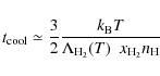
where
For gas at the beginning of the cooling branch,
![]() and
and
![]() ,
giving
,
giving
![]() yr (
yr (![]() in cm-3).
In the mean-density case (see phase diagram in Fig. 2),
in cm-3).
In the mean-density case (see phase diagram in Fig. 2),
![]() ,
while in the high-density region
(see phase diagram in Fig. 5),
,
while in the high-density region
(see phase diagram in Fig. 5),
![]() .
This translates into a characteristic cooling time of
.
This translates into a characteristic cooling time of ![]()
![]() for the former case and
for the former case and ![]()
![]() for the
latter.
for the
latter.
These estimates show the relevance of following the full cooling branch when simulating star formation at high redshift in regions of mean density, because the characteristic cooling times are a substantial fraction of the Hubble time. This problem is less severe for simulations of high-density peaks, in which the timescales are much shorter.
If one considers a
![]() halo at
halo at ![]() ,
its
average gas number density is of the order of
,
its
average gas number density is of the order of ![]()
![]() (being
(being ![]() the mean molecular weight), its virial temperature
the mean molecular weight), its virial temperature
![]() K and its cooling time
K and its cooling time
![]() -
-
![]() for an H2 fraction of 10-2-10-5, respectively.
The same halo at redshift
for an H2 fraction of 10-2-10-5, respectively.
The same halo at redshift ![]() would have an average gas number
density of
would have an average gas number
density of ![]()
![]() ,
,
![]() K, and
K, and
![]() -
-
![]() .
This means not only that objects of similar mass cool (and thus harbor
star formation) on very different timescales according to their
environment, but also that gas in high-redshift haloes can collapse and fragment much faster than in low-redshift ones, because its cooling capabilities are more efficient.
.
This means not only that objects of similar mass cool (and thus harbor
star formation) on very different timescales according to their
environment, but also that gas in high-redshift haloes can collapse and fragment much faster than in low-redshift ones, because its cooling capabilities are more efficient.
For these reasons, though low-density thresholds can be useful tools to reproduce empirical surface-density relations, such as the Kennicutt-Schmidt law (Schaye & Dalla Vecchia 2008; Springel & Hernquist 2003; Kennicutt 1998), physical insights can rely only on high-density thresholds. Indeed, imposing star formation events before the isothermal peak is reached could result in an artificially high-redshift for the onset of star formation.
For the test cases presented in this paper, the value adopted for the
high-density threshold is
![]() ,
well beyond the
isothermal peak of the gas. This allows a correct estimate
of the relevant timescales, as the gas spends most of the time in the
isothermal phase.
In addition, following the evolution of the gas to higher densities
allows higher resolution of, e.g., the morphology and disk
galaxy structure (Saitoh et al. 2008), the clumpiness of
the gas, and the features of the interstellar or intergalactic medium.
On the other hand, running high-density threshold simulations to
the present age (z=0) is computationally very challenging because of
the extremely short timescales involved in the calculations.
Only simulations performed with a low-density threshold are
currently run to z=0 and fine-tuned to reproduce the observed
low-redshift evolution of the star formation density.
,
well beyond the
isothermal peak of the gas. This allows a correct estimate
of the relevant timescales, as the gas spends most of the time in the
isothermal phase.
In addition, following the evolution of the gas to higher densities
allows higher resolution of, e.g., the morphology and disk
galaxy structure (Saitoh et al. 2008), the clumpiness of
the gas, and the features of the interstellar or intergalactic medium.
On the other hand, running high-density threshold simulations to
the present age (z=0) is computationally very challenging because of
the extremely short timescales involved in the calculations.
Only simulations performed with a low-density threshold are
currently run to z=0 and fine-tuned to reproduce the observed
low-redshift evolution of the star formation density.
We note that the mean-density region, because of
its small dimensions, lacks massive haloes.
In larger simulations, we expect to find rarer, larger, haloes, which can
grow faster and host star formation in ![]()
![]() -
-
![]() haloes.
haloes.
We have performed high-resolution, three-dimensional, N-body/SPH simulations including non-equilibrium atomic and molecular chemistry, star formation prescriptions, and feedback effects to investigate the onset of primordial star formation. We have studied how the primordial star formation rate changes according to different gas-density threshold, cosmological parameters, and simulation set-ups. Our main findings are summarized in the following:
-
The typical low-density thresholds (below
 )
are inadequate for describing star formation episodes in mean regions
of the universe at high redshift. To correctly estimate the onset
of star formation, high-density thresholds are necessary.
)
are inadequate for describing star formation episodes in mean regions
of the universe at high redshift. To correctly estimate the onset
of star formation, high-density thresholds are necessary.
-
In rare, high-density peaks, the density can be higher than
the usual low-density thresholds from very early times,
therefore these prescriptions are not physically meaningful. Density
thresholds lying beyond the isothermal peak (several particles per
cm3, in our case) are still required: they should satisfy the Bate & Burkert (1997) requirement (N at least
 )
and Eq. (6) of Sect. 2. However, as long as they are beyond the isothermal peak, given the faster evolution in the phase diagram of the cooling particles in dense environments, the very exact value is not crucial.
)
and Eq. (6) of Sect. 2. However, as long as they are beyond the isothermal peak, given the faster evolution in the phase diagram of the cooling particles in dense environments, the very exact value is not crucial.
-
Different values of the threshold and the cosmological parameters
can cause the onset of star formation at very different epochs:
with a low-density threshold (
 ), star formation
starts at
), star formation
starts at  -31 (depending on the cosmology), while
high-density threshold models (
)
predict a
much later onset, at
-31 (depending on the cosmology), while
high-density threshold models (
)
predict a
much later onset, at  -16 (depending on the cosmology).
-
Performing primordial, rare, high-density region simulations within
the high-density threshold model, we find that the local star
formation can set in as early as
 .
.
We conclude by adding a few comments on the meaning of the term ``onset of star formation''.
From a purely physical point of view, the onset of star formation occurs when the proton-proton nuclear reactions ignite in a collapsed, dense core. Nowadays, in numerical simulations of cosmic structure evolution, this definition cannot be adopted, since it is not feasible to follow and resolve the behaviour of the gas on the very large range of scales involved. Therefore, the onset of star formation is meant as the attainment of a certain density threshold: once SPH particles reach it, they are assumed to be dense enough to collapse and to host star formation.
This threshold can be viewed as a point of no return, because it imposes a limit above which the natural gas evolution is strongly altered by star production and feedback effects.
The time when the threshold is reached and the time when the actual star formation takes place are typically not the same, but if the threshold is set appropriately, as discussed in the present work, they become very similar.
Broadly speaking, one could consider assigning a simple prescription to standard numerical simulations based on the typical delay time of gas in fall. In this way, the onset of star formation could be easily corrected without implementing high-density thresholds or molecular evolution.
In practice, this is not a trivial task: the time spent in the isothermal regime depends on numerous ``environmental'' factors, so different simulations with different initial conditions will be affected differently, according to their particular features. However, as an estimate, a typical free-fall time of ![]()
![]() is the one we expect in correspondence of
is the one we expect in correspondence of ![]()
![]() (conventional low-density thresholds).
(conventional low-density thresholds).
Throughout this paper, we have considered the onset of star formation to be the attainment of the density threshold, provided that the Jeans mass is resolved by a ``large'' number of SPH particles and the isothermal peak in the phase diagram is resolved (and we have seen in Sects. 2 and 4 that the latter two conditions are strongly related).
Acknowledgements
We acknowledge useful discussions with James Bolton, Massimo Ricotti, Cecilia Scannapieco, Volker Springel, Romain Teyssier, Michele Trenti, Simon D. M. White and John Wise. N.Y. thanks financial support from Grants-in-Aid for Young Scientists S from JSPS (20674003). We also acknowledge the anonymous referee for stimulating comments on the paper. The simulations were performed using the machines of the Max Planck Society computing center, Garching (Rechenzentrum-Garching) and of the Max-Planck-Institut für Astrophysik. For the bibliografic research we have made use of the tools offered by the NASA Astrophysics Data System and by the JSTOR Archive.
References
- Abel, T., Bryan, G. L., & Norman, M. L. 2002, Science, 295, 93 [NASA ADS] [CrossRef]
- Bate, M. R., & Burkert, A. 1997, MNRAS, 288, 1060 [NASA ADS]
- Bate, M. R., Bonnell, I. A., & Price, N. M. 1995, MNRAS, 277, 362 [NASA ADS]
- Bolton, J. S., & Haehnelt, M. G. 2007, MNRAS, 382, 325 [NASA ADS] [CrossRef] (In the text)
- Brax, P. H., & Martin, J. 1999, Phys. Lett. B, 468, 40 [NASA ADS] [CrossRef] (In the text)
- Bromm, V., & Larson, R. B. 2004, ARA&A, 42, 79 [NASA ADS] [CrossRef]
- Bromm, V., Coppi, P. S., & Larson, R. B. 2002, ApJ, 564, 23 [NASA ADS] [CrossRef]
- Cen, R., & Ostriker, J. P. 1992, ApJ, 399, L113 [NASA ADS] [CrossRef]
- Ciardi, B., & Ferrara, A. 2005, Space Sci. Rev., 116, 625 [NASA ADS] [CrossRef] (In the text)
- Crociani, D., Viel, M., Moscardini, L., Bartelmann, M., & Meneghetti, M. 2008, MNRAS, 385, 728 [NASA ADS] [CrossRef] (In the text)
- Dalla Vecchia, C., & Schaye, J. 2008, MNRAS, 387, 1431 [NASA ADS] [CrossRef]
- Einstein, A. 1917, Sitzungsberichte der Königlich Preußischen Akademie der Wissenschaften, Berlin, 142 (In the text)
- Evrard, A. E. 1988, MNRAS, 235, 911 [NASA ADS] (In the text)
- Galli, D., & Palla, F. 1998, A&A, 335, 403 [NASA ADS] (In the text)
- Gao, L., Yoshida, N., Abel, T., et al. 2007, MNRAS, 378, 449 [NASA ADS] [CrossRef]
- Governato, F., Willman, B., Mayer, L., et al. 2007, MNRAS, 374, 1479 [NASA ADS] [CrossRef]
- Gunn, J. E., & Gott, J. R. I. 1972, ApJ, 176, 1 [NASA ADS] [CrossRef] (In the text)
- Hernquist, L., & Katz, N. 1989, ApJS, 70, 419 [NASA ADS] [CrossRef] (In the text)
- Hinshaw, G., Weiland, J. L., Hill, R. S., et al. 2008, ArXiv e-prints, 803 (In the text)
- Hollenbach, D., & McKee, C. F. 1979, ApJS, 41, 555 [NASA ADS] [CrossRef]
- Inutsuka, S.-I., & Miyama, S. M. 1992, ApJ, 388, 392 [NASA ADS] [CrossRef]
- Jeans, J. H. 1902, Phil. Trans., 199, A 1 (In the text)
- Katz, N. 1992, ApJ, 391, 502 [NASA ADS] [CrossRef]
- Katz, N., Weinberg, D. H., & Hernquist, L. 1996, ApJS, 105, 19 [NASA ADS] [CrossRef]
- Kennicutt, Jr., R. C. 1998, ARA&A, 36, 189 [NASA ADS] [CrossRef]
- Larson, R. B. 1998, MNRAS, 301, 569 [NASA ADS] [CrossRef]
- Maio, U., Dolag, K., Meneghetti, M., et al. 2006, MNRAS, 373, 869 [NASA ADS] [CrossRef] (In the text)
- Maio, U., Dolag, K., Ciardi, B., & Tornatore, L. 2007, MNRAS, 379, 963 [NASA ADS] [CrossRef] (In the text)
- Maio, U., Ciardi, B., Dolag, K., & Tornatore, L. 2008, in First Stars III, ed. B. W. O'Shea, & A. Heger, AIP Conf. Ser., 990, 33
- Nakamura, F., & Umemura, M. 2001, ApJ, 548, 19 [NASA ADS] [CrossRef]
- Navarro, J. F., & White, S. D. M. 1993, MNRAS, 265, 271 [NASA ADS]
- Omukai, K., & Palla, F. 2003, ApJ, 589, 677 [NASA ADS] [CrossRef]
- Pawlik, A. H., Schaye, J., & van Scherpenzeel, E. 2009, MNRAS, 394, 1812 [NASA ADS] [CrossRef]
- Peebles, P. J. E. 1974, ApJ, 189, L51 [NASA ADS] [CrossRef]
- Peebles, P. J. E., & Dicke, R. H. 1968, ApJ, 154, 891 [NASA ADS] [CrossRef]
- Peebles, P. J., & Ratra, B. 2003, Rev. Mod. Phys., 75, 559 [NASA ADS] [CrossRef] (In the text)
- Ratra, B., & Peebles, P. J. E. 1988, Phys. Rev. D, 37, 3406 [NASA ADS] [CrossRef] (In the text)
- Ricotti, M., Gnedin, N. Y., & Shull, J. M. 2002a, ApJ, 575, 33 [NASA ADS] [CrossRef]
- Ricotti, M., Gnedin, N. Y., & Shull, J. M. 2002b, ApJ, 575, 49 [NASA ADS] [CrossRef]
- Ricotti, M., Gnedin, N. Y., & Shull, J. M. 2008, ArXiv e-prints, 802
- Saitoh, T. R., Daisaka, H., Kokubo, E., et al. 2008, PASJ, 60, 667 [NASA ADS] (In the text)
- Saslaw, W. C., & Zipoy, D. 1967, Nature, 216, 976 [CrossRef]
- Scannapieco, C., Tissera, P. B., White, S. D. M., & Springel, V. 2005, MNRAS, 364, 552 [NASA ADS]
- Schaye, J., & Dalla Vecchia, C. 2008, MNRAS, 383, 1210 [NASA ADS] [CrossRef]
- Schwarzschild, M., & Spitzer, L. 1953, The Observatory, 73, 77 [NASA ADS]
- Springel, V. 2005, MNRAS, 364, 1105 [NASA ADS] [CrossRef] (In the text)
- Springel, V., & Hernquist, L. 2003, MNRAS, 339, 289 [NASA ADS] [CrossRef]
- Tegmark, M., Silk, J., Rees, M. J., et al. 1997, ApJ, 474, 1 [NASA ADS] [CrossRef]
- Tornatore, L., Borgani, S., Dolag, K., & Matteucci, F. 2007a, MNRAS, 382, 1050 [NASA ADS] (In the text)
- Tornatore, L., Ferrara, A., & Schneider, R. 2007b, MNRAS, 382, 945 [NASA ADS]
- Trenti, M., & Stiavelli, M. 2009, ApJ, 694, 879 [NASA ADS] [CrossRef]
- Truelove, J. K., Klein, R. I., McKee, C. F., et al. 1997, ApJ, 489, L179 [NASA ADS] [CrossRef]
- Wetterich, C. 1988, Nucl. Phys. B, 302, 668 [NASA ADS] [CrossRef] (In the text)
- Whalen, D., O'Shea, B. W., Smidt, J., & Norman, M. L. 2008, ApJ, 679, 925 [NASA ADS] [CrossRef]
- White, S. D. M., & Rees, M. J. 1978, MNRAS, 183, 341 [NASA ADS]
- Wiersma, R. P. C., Schaye, J., Theuns, T., Dalla Vecchia, C., & Tornatore, L. 2009, ArXiv e-prints (In the text)
- Wise, J. H., & Abel, T. 2007, ApJ, 665, 899 [NASA ADS] [CrossRef]
- Wise, J. H., & Abel, T. 2008, ApJ, 685, 40 [NASA ADS] [CrossRef]
- Yoshida, N., Abel, T., Hernquist, L., & Sugiyama, N. 2003, ApJ, 592, 645 [NASA ADS] [CrossRef]
- Yoshida, N., Omukai, K., Hernquist, L., & Abel, T. 2006, ApJ, 652, 6 [NASA ADS] [CrossRef]
- Yoshida, N., Omukai, K., & Hernquist, L. 2007, ApJ, 667, L117 [NASA ADS] [CrossRef]
Footnotes
- ... limit
![[*]](/icons/foot_motif.png)
-
This widely-used approximation is appropriate as, according to the
classical spherical ``top-hat'' model, a virialized object has a total
mass density of
 times the critical density, which
corresponds, on average, to a total number density of
times the critical density, which
corresponds, on average, to a total number density of
 at
at  ,
for a WMAP5 cosmology and a mean molecular
weight
,
for a WMAP5 cosmology and a mean molecular
weight
 .
The transition to a high-density statistical equilibrium
regime happens at critical number densities of
.
The transition to a high-density statistical equilibrium
regime happens at critical number densities of
 .
.
- ...
stars
- To reduce the computation time for calculations of fragmentation sometimes, particles with densities above the threshold are replaced by ``sink'' particles (Bate et al. 1995).
- ... length
- The definition of smoothing length may vary from authors to authors. It is sometimes meant to be the width of the SPH smoothing kernel, but other times the length scale on which the SPH smoothing kernel becomes zero.
- ... softening
- The comoving gravitational softening is usually estimated as 1/20 or 1/30 the mean inter-particle separation.
- ...(Gao et al. 2007)
- We use the ``R4'' initial conditions presented there.
- ...Galli & Palla (1998)
-
We assume a primordial neutral gas with residual electron and H+fractions
 ,
H2 fraction
,
H2 fraction
 ,
H2+ fraction
,
H2+ fraction
 ,
D fraction
,
D fraction
 ,
HD fraction
,
HD fraction
 ,
D+ fraction
,
D+ fraction
 ,
HeH+ fraction
,
HeH+ fraction
 .
.
- ... index
-
By effective index of the gas,
 ,
we mean
,
we mean
 ,
with P pressure and
,
with P pressure and  density.
This is simply related to the politropic index.
density.
This is simply related to the politropic index.
- ...Galli & Palla (1998)
-
The initial abundances (at z=399) are consistent with a primordial
neutral plasma having residual electron and H+ fractions of
 ,
H2 fraction
,
H2 fraction
 ,
H2+ fraction
,
H2+ fraction
 ,
D fraction
,
D fraction
 ,
D+ fraction
,
D+ fraction
 ,
HD fraction
,
HD fraction
 ,
HeH+ fraction
,
HeH+ fraction
 .
.
All Tables
Table 1: Parameters adopted for the simulations.
All Figures
| |
Figure 1:
First, second, and third column are respectively
temperature, density, and molecule maps.
The first two rows refer to the mean-region simulation at redshift
12.17 ( top) and 30.16 ( bottom).
The box size is 1 Mpc comoving.
The last two rows refer to the high-density region at redshift
50 ( top) and 70 ( bottom).
The region size is |
| Open with DEXTER | |
| In the text | |
| |
Figure 2:
Upper panel:
phase diagram at redshift z=12.17 (just before the onset of
star formation) for the wmap5-ht simulation.
The vertical straight lines indicate a
low physical critical density threshold of
|
| Open with DEXTER | |
| In the text | |
| |
Figure 3: Evolution of the ten most massive haloes in the wmap5-ht cosmological simulation (dotted lines). The redshift at which the first star forms in each halo is indicated by the filled star symbols. After that, star formation continues along the solid lines. |
| Open with DEXTER | |
| In the text | |
| |
Figure 4: Star formation rate as a function of redshift for the different models, from left to right: WMAP5 cosmology and high-density threshold (solid red line), standard cosmology and high-density threshold (dotted blue line), WMAP5 cosmology and low-density threshold (dot-dashed black line), standard cosmology and low-density threshold (long-dashed-short-dashed magenta line). The green short-dashed line refers to the simulation of the high-density region with standard parameters and high-density threshold. |
| Open with DEXTER | |
| In the text | |
| |
Figure 5:
Upper panel:
phase diagram at redshift z=45.41 for the high-density region
simulation for a purely non-equilibrium chemistry run (i.e. without
star formation).
The vertical straight lines show physical critical-density threshold
of
|
| Open with DEXTER | |
| In the text | |
Copyright ESO 2009
Current usage metrics show cumulative count of Article Views (full-text article views including HTML views, PDF and ePub downloads, according to the available data) and Abstracts Views on Vision4Press platform.
Data correspond to usage on the plateform after 2015. The current usage metrics is available 48-96 hours after online publication and is updated daily on week days.
Initial download of the metrics may take a while.