| Issue |
A&A
Volume 497, Number 2, April II 2009
|
|
|---|---|---|
| Page(s) | 521 - 524 | |
| Section | The Sun | |
| DOI | https://doi.org/10.1051/0004-6361/200811107 | |
| Published online | 05 March 2009 | |
Global prominence oscillations
(Research Note)
U. Anzer
Max-Planck-Institut für Astrophysik, Karl-Schwarzschild-Str. 1, 85740 Garching, Germany
Received 8 October 2008 / Accepted 28 January 2009
Abstract
Aims. The question of the different oscillation periods for global modes of quiescent prominences is discussed.
Methods. Simple 1D prominence configurations are used to describe the magnetohydrostatic equilibrium and their oscillations for small amplitudes.
Results. Three basic modes of oscillations were found and their periods as a function of the magnetic field configuration and the assumed geometry are given.
Key words: Sun: prominences
1 Introduction
Oscillatory motions of solar prominences have been observed for a long time, going back to the early investigations of Harvey (1969). The observed velocity amplitudes of the oscillations range from a few km s-1 up to around 100 km s-1. Many theoretical investigations which try to model these oscillations have been presented over the years. A summary of these theoretical models can be found in the review of Ballester (2006), which also gives in some detail the relevant observations.
As is well known, prominences are massive cool structures in the solar corona which have to be supported against gravity by a sufficiently strong upward force. The most obvious force is the Lorentz force of the associated magnetic field. This aspect has to be taken into account in the basic equilibrium models. Another important point for the oscillation modelling is the fact that the prominence can interact with its coronal surroundings; this will have a non-negligible effect on the the different modes.
Most of the existing models do not fulfill all these requiremnts simultaneously. There is for example a paper by Oliver et al. (1992) where the full magneto-hydrostatic (MHS) equilibrium is properly treated. But only internal modes are considered by prescribing vanishing velocities at the prominence-corona interface. This then means that the effects of the surrounding corona are ignored. On the other hand a study by Joarder & Roberts (1992) allows both for internal and global oscillations (i.e. modes where the prominence and the corona are involved). But in this investigation gravity is completely neglected and the magnetic support not treated correctly.
There are also a few models which aim at including the effects of gravity and of the surrounding corona simultaneously, e.g. an investigation by Joarder & Roberts (1993a) and another by Oliver et al. (1993). We postpone the comparison of these models to our new results to Sect. 6. In the present investigation we look at oscillations of prominences which are in MHS equilibrium and which also can interact with the surrounding coronal magnetic field. In order to make this rather complex problem tractable for analytical investigations we have to make some rather strong simplifications which will be described in the following sections. In Sect. 2 we present our basic prominence model and calculate the different oscillatory modes. In Sect. 3 we mention some other types of modelling and in Sect. 4 we describe possible applications of our results. Sect. 5 briefly outlines the consequences of magnetic shear. Sect. 6 gives the conclusions.
2 Global oscillations
For our modelling we use the simplest configuration of a
prominence in MHS equilibrium. We take a 1D slab model of the
type proposed earlier by Kippenhahn & Schlüter
(1957); more details of such slab models can be found in the paper
by Heinzel & Anzer (2005)
and models that allow for vertical variations have been
discussed
by Hood & Anzer (1990). But in the present investigation we
adopt the most simple configuration.
For the description we use Cartesian
coordinates with x normal to the slab, y along its axis
and z pointing vertically upward. In this model all physical
quantities are assumed to vary only in the x-direction. For the
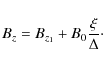
magnetic field inside the prominence we take the relation
| (1) |
with
 and Bz(x) being antisymmetric with
respect to x = 0. The prominence boundaries are placed at the
positions
and Bz(x) being antisymmetric with
respect to x = 0. The prominence boundaries are placed at the
positions
 .
If we then denote by
.
If we then denote by  the
density and by g the solar gravity we obtain the following
equation for vertical equilibrium:
the
density and by g the solar gravity we obtain the following
equation for vertical equilibrium:
 |
(2) |
and the column mass, M, is obtained as
 |
(3) |
Equation (2) can be integrated and leads to
 |
(4) |
where Bz1 = Bz(D/2) has been taken.
Note: Eq. (4) holds for any temperature distribution present inside the prominence. More details about the internal structure of the prominence can be found in Heinzel & Anzer (2005).
Outside of the prominence we have a low  plasma for which we
assume a potential magnetic field which is anchored in the solar
photospere. In order to make the equilibrium configuration tractable
for an analytical investigation we replace the photosphere by two
vertical solid boundaries placed at
plasma for which we
assume a potential magnetic field which is anchored in the solar
photospere. In order to make the equilibrium configuration tractable
for an analytical investigation we replace the photosphere by two
vertical solid boundaries placed at
 .
In this case
the coronal field is given by
.
In this case
the coronal field is given by
| (5) |
This configuration is shown in Fig.1.
![\begin{figure}
\par\includegraphics[width=8.8cm]{1107fig1.eps}
\par\end{figure}](/articles/aa/full_html/2009/14/aa11107-08/img11.png) |
Figure 1: Sketch of the prominence configuration used for the present modelling. Note that the true width of the prominence is much smaller than drawn here. |
| Open with DEXTER | |
For this type of slab model one has 3 fundamental oscillatory modes:
horizontal motion in x-direction, horizontal motion in y-direction
and vertical oscillations. For all of the fundamental modes
the prominence will move as a solid body without any internal
deformations. We now denote by  the displacement in each of
these modes and then obtain the general equation of motion:
the displacement in each of
these modes and then obtain the general equation of motion:
 |
(6) |
where
 is the restoring force which has to be determined
for each of the 3 modes individually.
is the restoring force which has to be determined
for each of the 3 modes individually.
2.1 Oscillations in the x-direction
The restoring force in this case is the difference in magnetic pressure on the right and left side of the prominence. Because of flux conservation one has the relation |
(7) |
With this one then obtains for F the expression
 |
(8) |
Making use of Eqs. (4) and (6) we arrive at the oscillation equation given by
 |
(9) |
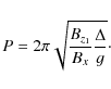
and with this we obtain the period of the oscillations as
 |
(10) |
2.2 Oscillations in the y- and z-direction
For the oscillations in the y-direction the restoring force results from the magnetic tension of the stretched field lines. We now have |
(11) |
leading to a period of
 |
(12) |
For the oscillations in the z-direction the restoration is again achieved by field line stretching. In this case we obtain
 |
(13) |
Taking the MHS equilibrium as given in Eq. (4) into account we then arrive for the restoring force at the same expression as for the y-oscillations (i.e.
is also given by Eq. (11)) and therefore
the periods are the same. It is interesting to note that although
the physical situation is quite different for y- and
z-oscillations,
the periods turn out to be identical. But for
configurations
with magnetic shear this is no longer the case (see the discussion in
Sect. 5).
2.3 Interpretations
Equations (10) and (12) are actually those of a swinging pendulum which has a length of ,
respectively
,
respectively
 .
At first sight this result might seem somewhat surprising since the
restoring force in all cases is of magnetic origin and therefore
one would expect the field strength to be the determing factor. But
since in our MHS equilibrium the field is directly related to gravity
these results are very plausible.
An alternative interpretation based upon a model consisting of an
isolated blob hanging in a magnetic string has been proposed by
Roberts (1991). This modelling gives the
same result as Eq. (12) for vertical oscillations.
Much more detailed discussions of the
so-called string modes can be found in Joarder &
Roberts (1992, 1993a) and Roberts & Joarder (1994).
In our modelling the quantity
entering Eq. (12) can be interpreted as the total depth of the
field line dips; the quantity
has no
obvious physical meaning. Both observations and prominence modelling
indicate that in general the field line inclination is rather small
and therfore
.
At first sight this result might seem somewhat surprising since the
restoring force in all cases is of magnetic origin and therefore
one would expect the field strength to be the determing factor. But
since in our MHS equilibrium the field is directly related to gravity
these results are very plausible.
An alternative interpretation based upon a model consisting of an
isolated blob hanging in a magnetic string has been proposed by
Roberts (1991). This modelling gives the
same result as Eq. (12) for vertical oscillations.
Much more detailed discussions of the
so-called string modes can be found in Joarder &
Roberts (1992, 1993a) and Roberts & Joarder (1994).
In our modelling the quantity
entering Eq. (12) can be interpreted as the total depth of the
field line dips; the quantity
has no
obvious physical meaning. Both observations and prominence modelling
indicate that in general the field line inclination is rather small
and therfore
 will hold. From this we conclude
that in most cases the periods of the x-oscillations will be longer
than those of the other two modes. As a representative example we take
Bz1/Bx = 0.1 and
will hold. From this we conclude
that in most cases the periods of the x-oscillations will be longer
than those of the other two modes. As a representative example we take
Bz1/Bx = 0.1 and
 km and then obtain typical
values for the periods of 200 min for x-oscillations and 20 min for
the other cases. If the field lines are shorter,
and
km and then obtain typical
values for the periods of 200 min for x-oscillations and 20 min for
the other cases. If the field lines are shorter,
and  smaller, then
the periods will be reduced correspondingly.
smaller, then
the periods will be reduced correspondingly.
3 Pressure driven oscillations
One could also consider the alternative possibility that
the coronal magnetic field is so strong that the prominence
cannot distort this field by a large amount. If we further
assume that the field inside the prominence is basically
horizontal (i.e. has only negligible dips) then the only restoring
force will be the difference in coronal gas pressure between
the left and right side of the slab. This force is given by
 |
(14) |
and therefore one has
 |
(15) |
where
 is the unperturbed coronal pressure. Since in this
particular case the pressure inside the prominence,
and therefore also the density
because of an assumed constant temperature,
are uniform one obtains the relation
is the unperturbed coronal pressure. Since in this
particular case the pressure inside the prominence,
and therefore also the density
because of an assumed constant temperature,
are uniform one obtains the relation
| (16) |
with
 denoting the prominence density and D its full width.
For the equilibrium one also needs
denoting the prominence density and D its full width.
For the equilibrium one also needs
| (17) |
We also set
 |
(18) |
where
 is the sound velocity inside the cool slab. Making use
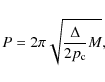
of these relations we arrive at the equation
is the sound velocity inside the cool slab. Making use
of these relations we arrive at the equation
 |
(19) |
for the period.
Note: this period is identical to that found by Joarder & Roberts (1992) for the case of slow kink modes.
If we now take some typical values for the configuration with
 dyn/cm2,
M = 10-4 g/cm2 and
T = 6000 K
we can derive the following numbers:
dyn/cm2,
M = 10-4 g/cm2 and
T = 6000 K
we can derive the following numbers:
 g/cm3,
 km s-1 and
D = 14 000 km.
Together with the value
for
which we used in the previous section of 100 000 km we
get in this case an oscillation period of P = 430 min. This value is much
larger than any period observed in prominences.
The values for the period could be reduced by assuming higher temperatures
which will result in higher sound velocities and also smaller column masses
which correspond to smaller values of D (e.g. a temperature of
10 000 K and a column mass of
km s-1 and
D = 14 000 km.
Together with the value
for
which we used in the previous section of 100 000 km we
get in this case an oscillation period of P = 430 min. This value is much
larger than any period observed in prominences.
The values for the period could be reduced by assuming higher temperatures
which will result in higher sound velocities and also smaller column masses
which correspond to smaller values of D (e.g. a temperature of
10 000 K and a column mass of
 g/cm2 gives a
period of 245 min.).
g/cm2 gives a
period of 245 min.).
But a more serious problem with this type of models is the fact that
they require extremely large coronal magnetic fields. In order to be
able to neglect the effects of hydrostatic layering inside the slab the
magnetic field has to be horizontal to a high degree of accuracy. If
we take for example this constraint as
 then
Eq. (4) together with a column mass of 10-4 g/cm2 leads to
the condition
then
Eq. (4) together with a column mass of 10-4 g/cm2 leads to
the condition
| (20) |
Therefore one has to conclude that only those prominences with such very large magnetic fields will allow this kind of simplified modelling.
4 Consequences for the diagnosing of prominences
The study of prominence oscillations can give us detailed insight into the physics of prominences. The present status of this field of so-called prominence seismology has been summarised in the reviews of Oliver (2004) and Ballester (2006). Interesting new observations can be found in the papers of Régnier et al. (2001) and Pouget et al. (2006). Our new modelling of of the global oscillations can then also be used to derive the basic parameters of solar prominences. The important point is that both the periods of normal and tangential oscillations must be measured. If we denote by P1 the period of oscillations in the x-direction and by P2 that of oscillations either in the y- or in z-direction we obtain from Eqs. (10) and (12) the relation |
(21) |
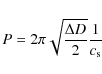
We can determine in this way the field line inclination at the prominence boundary. One also gets
 |
(22) |
which gives an estimate of the length of the coronal field lines.
In addition the observations of prominences on the limb
seen in the H line allow a determination of the column
mass, M (Gouttebroze et al. 1994).
With this knowledge we can then also calculate the strength of the
magnetic field as
line allow a determination of the column
mass, M (Gouttebroze et al. 1994).
With this knowledge we can then also calculate the strength of the
magnetic field as
 |
(23) |
This shows that for our models all global physical parameters can be derived, in principle. But it is important to note that for this procedure the knowledge of both P1 and P2 of the prominence under investigation will be needed.
5 Effects resulting from magnetic shear
So far we have considered only unsheared prominence configurations in order to make our analysis as simple and transparent as possible. But the observations of quiescent prominences indicate the presence of strong magnetic shear (see e.g. Leroy et al. 1984). Therefore we shall now briefly outline what consequences the magnetic shear has on our modelling.
We model this by adding a constant y-component, By, to the
equilibrium field. With this then the horizontal field strength is
given by
 |
(24) |
and the shear is quantified by the parameter
 .
With this definition the length of the horizontal field to the boundary
now amounts to
.
With this definition the length of the horizontal field to the boundary
now amounts to
 and the column mass as
measured along the field is given by
and the column mass as
measured along the field is given by
 .
With this modified configuration we find the following three basic
types of oscillations: motions along the horizontal field direction, those
perpendicular to it, and verical ones. The first two modes correspond
respecively to the x- and y-oscillation of the unsheared case. We
found that the equations for the periods of the first two types of
oscillations are the same as previously calculated but with Bx
replaced by Bh and M replaced by M1. In the equation for the
vertical mode an additional factor
.
With this modified configuration we find the following three basic
types of oscillations: motions along the horizontal field direction, those
perpendicular to it, and verical ones. The first two modes correspond
respecively to the x- and y-oscillation of the unsheared case. We
found that the equations for the periods of the first two types of
oscillations are the same as previously calculated but with Bx
replaced by Bh and M replaced by M1. In the equation for the
vertical mode an additional factor
 has to introduced.
If we keep the values of Bx and
fixed we get the following
scaling laws for the periods: the mode along the field is proportional
to ,
the vertical one to
,
and the perpendicular
mode is unchanged. This result implies that the periods of the first
two modes are increased and the third one is not affected by the
shear. Very long period oscillations resulting from a strong
magnetic shearing were also predicted by Joarder & Roberts (1993b).
has to introduced.
If we keep the values of Bx and
fixed we get the following
scaling laws for the periods: the mode along the field is proportional
to ,
the vertical one to
,
and the perpendicular
mode is unchanged. This result implies that the periods of the first
two modes are increased and the third one is not affected by the
shear. Very long period oscillations resulting from a strong
magnetic shearing were also predicted by Joarder & Roberts (1993b).
6 Conclusions
The prominence models considered in this paper are highly simplified configurations. Still, they can be taken as reasonable first order approximations to real prominence slabs. The assumption that the slab is very extended along the direction of the prominence axis is acceptable. But assuming also that the prominence extension in height is very large is less appropriate. There is in particular the aspect that the solar surface represents a solid lower boundary. This can influence the vertical oscillations. If we assume that the prominence does not extend down to the surface then the magnetic field which crosses the region below the prominence will provide some additional restoring force. This means that the periods calculated from our Eq. (12) are actually overestimates and the true periods of vertical oscillations will be smaller. The reduction of the period will depend on the details of the prominence geometry.Our simple analytical results given by Eqs. (10) and (12) can also be compared with other approaches given in the literature. Joarder & Roberts (1993a) investigated oscillations that occur in the prominence model of Menzel. They obtained periods for the different modes ranging from 4 min up to 48 min. But these results have to be taken with caution since the Menzel model is not a realistic model for prominences and a comparison with our results is not so meaningful. The only other investigation which takes both gravity and the coronal surrounding into account is that of Oliver et al. (1992). Because of the large complexity they had to treat the problem numerically and thus could only calculate the oscillations for one prominence. For the fundamental modes they found P = 70 min for horizontal oscillations and P = 13 min for vertical ones. Using our Eqs. (10) and (12) and taking their prominence model we get 78 min, resp. 15 min for the basic modes. Therefore our simple, but analytical, model gives similar results. From this we conclude that if one is interested in the oscillations of the prominence as a whole our simple treatment is fully adequate.
In addition we have the problem of prominence fine structure. But as long as these fine structures are small compared tothe prominence extensions one can consider all the quantities used here as mean values. With this then the global aspects of the oscillations will be described appropriately. But if one considers localised modes of oscillations then the fine structures are of primary interest. Such a fine structure modelling has recently be done by Joarder et al. (1997).
The other crucial point is that the coronal magnetic field is assumed to have straight field lines which are anchored in two vertical rigid boundaries. In reality the field has to bend over to connect to the solar surface. This bending is completely ignored in our modelling, whereas the photospheric line-tying is included. Therefore our estimates for the magnetic restoring forces are only approximations. Unfortunately the modelling based upon more realisic curved field configurations cannot be done in a simple analytic way.
We also want to point out that our modelling concentrates on the global modes and therefore it will give us information on the overall magnetic field structure as well as the total prominence mass. For complementary information concerning the interior of the prominence the internal modes of oscillation which were briefly lined out in the introduction should be used.
Acknowledgements
I would like to thank the referee, Bernie Roberts, for his comments which helped to improve the paper considerably.
References
- Ballester, J. L. 2006, Phil. Trans. R. Soc. A 364, 405 In the text
- Gouttebroze, P., Heinzel, P., & Vial, J. C. 1994, A&AS, 99, 513 In the text
- Harvey, J. 1969, Ph.D. Thesis, University of Colorado, USA In the text
- Heinzel, P., & Anzer, U. 2005, in Solar Magnetic Phenomena, ed. A. Hanslmeier, A. Veronig, & M. Messerotti (Springer) ASSL, 320 115
- Hood, A. W., & Anzer, U. 1990, SP, 126, 117 In the text
- Joarder, P. S., & Roberts, B. 1992, A&A, 261, 625 In the text
- Joarder, P. S., & Roberts, B. 1993a, A&A, 273, 642 In the text
- Joarder, P. S., & Roberts, B. 1993b, A&A, 277, 225
- Joarder, P. S., Nakariakov, V. M., & Roberts, B. 1997, SP, 173, 81 In the text
- Kippenhahn, R., & Schlüter, A. 1957, Z. Astrophys., 43, 36 In the text
- Leroy, J. L., Bommier, V., & Sahal-Bréchot, S. 1984, A&A, 131, 33 In the text
- Oliver, R. 2004, in Proc. of SOHO 13, Palma de Mallorca, ESA SP-547, 175 In the text
- Oliver, R., Ballester, J. L., Hood, A. W., & Priest, E. R. 1992, ApJ, 400, 369 In the text
- Oliver, R., Ballester, J. L., Hood, A. W., & Priest, E. R. 1993, ApJ, 409, 809 In the text
- Pouget, G., Bocchialini, K., & Solomon, J. 2006, A&A, 450, 1189 In the text
- Régnier, S., Solomon, J., & Vial, J. C. 2001, A&A, 376, 292 In the text
- Roberts, B. 1991, Geophys. Astrophys. Fluid Dyn., 62, 83 In the text
- Roberts, B., & Joarder, P. S. 1994, in Proc. of 7th ESP meeting on Solar Physics, ed. G. Belvedere, M. Rodonò, & G. M. Simnett, LNP, 432, 173 In the text
All Figures
| |
Figure 1: Sketch of the prominence configuration used for the present modelling. Note that the true width of the prominence is much smaller than drawn here. |
| Open with DEXTER | |
| In the text | |
Copyright ESO 2009
Current usage metrics show cumulative count of Article Views (full-text article views including HTML views, PDF and ePub downloads, according to the available data) and Abstracts Views on Vision4Press platform.
Data correspond to usage on the plateform after 2015. The current usage metrics is available 48-96 hours after online publication and is updated daily on week days.
Initial download of the metrics may take a while.