| Issue |
A&A
Volume 502, Number 3, August II 2009
|
|
|---|---|---|
| Page(s) | 957 - 968 | |
| Section | The Sun | |
| DOI | https://doi.org/10.1051/0004-6361/200810899 | |
| Published online | 15 June 2009 | |
Analytical model of static coronal loops
J. Dudík1 - E. Dzifcáková1,2 - M. Karlický2 - A. Kulinová1,2
1 - Department of Astronomy, Physics of the Earth and Meteorology, Faculty of Mathematics, Physics and Informatics, Comenius University, Mlynská Dolina F2, 842 48 Bratislava, Slovak Republic
2 - Astronomical Institute of the Academy of Sciences of the Czech Republic, Fricova 298, 251 65 Ondrejov, Czech Republic
Received 9 September 2008 / Accepted 23 March 2009
Abstract
By solving the energy-equilibrium equation in the stationary case, we derive analytical formulae in the form of scaling laws for non-uniformly heated and gravitationally stratified coronal loops. The heating is assumed to be localized in the chromosphere and to exponentially decrease with increasing distance along the loop strand. This exponential behavior of the heating and pressure profiles implies that we need to use the mean-value theorem, and in turn fit the mean-value parameters of the scaling laws to the results of the numerical simulations. The radiative-loss function is approximated by a power-law function of the temperature, and its effect on the resulting scaling laws for coronal loops is studied. We find that this effect is more important than the effect of varying loop geometry. We also find that the difference in lengths of the different loop strands in a loop with expanding cross-section does not produce differences in the EUV emission of these strands significant enough to explain the observed narrowness of the coronal loops.
Key words: hydrodynamics - Sun: corona - Sun: UV radiation - stars: coronae
1 Introduction
Since the first observations of the solar corona in the extreme ultraviolet (EUV) and soft X-rays, it has been undeniably clear that the corona is a highly structured environment. The basic structural blocks observed mainly in active regions are coronal loops - thin, arch-like, or elongated cylindrical structures delineating magnetic field lines. Coronal loops are anchored in the solar chromosphere at one or both ends. The presence of EUV and X-ray emission from these coronal loops means that the loops are hot - their temperatures reach several million K. The fact that the physical mechanism(s) heating the corona has still not been successfully identified constitutes the coronal heating problem (e.g., Klimchuk 2006).
One approach to constraining the coronal heating problem is the direct physical modeling of the temperature and density structure of the coronal loops. Analytical models are an invaluable tool for accomplishing this task, even if they employ a number of simplifying assumptions. The most frequent assumption is that of static energy equilibrium. Further assumptions include the uniform pressure throughout the loop (e.g., Kuin & Martens 1982; Chiuderi et al. 1981; Rosner et al. 1978; Craig et al. 1978; Martens 2009) and uniform energy input (Vesecky et al. 1979), while others relax one or both of these assumptions (e.g., Aschwanden & Schrijver 2002; Wragg & Priest 1979; Serio et al. 1981). The stability of the static solutions have been extensively studied (e.g., Craig et al. 1982; Hood & Priest 1979,1980; Chiuderi et al. 1981; Antiochos 1979). Aschwanden & Tsiklauri (2009) demonstrated the feasibility of analytical models even for non-static situations corresponding to impulsively heated loops with subsequent cooling.
The usual solution to the energy balance equation in the static case is written in the form of scaling laws due to the over-specification of the boundary conditions (Martens 2009). The three most seminal papers on scaling laws are those of Rosner et al. (1978), Serio et al. (1981), and Aschwanden & Schrijver (2002). The first two of these papers assume a simplified radiative-loss function in the form of the temperature power-law with fixed parameters, while the latest uses the radiative-loss function of Tucker & Koren (1971). The effect of the radiative-loss function parameters on resulting scaling laws was studied by Kuin & Martens (1982) and Martens (2009), although only for the loops with uniform pressure. None of these papers treat the effects of varying loop geometry. However, the effect of the varying loop cross-sectional area on the temperature and density profiles of the coronal loops has been extensively studied (Aschwanden & Schrijver 2002; Martens 2009; Vesecky et al. 1979) and found to be small, even though the changes in temperature and density profiles act cumulatively to increase the differential emission measure near the loop apex (Vesecky et al. 1979).
We derive new analytical scaling laws for non-uniformly heated and gravitationally stratified coronal loops. These scaling laws are explicitly dependent on the parameters of the radiative-loss function, making them the most general scaling laws for coronal loops existing to date.
This paper is organized as follows. The assumptions and derivation of new scaling laws for coronal loops is given in Sect. 2. Discussion of different effects on the equilibrium solutions or resulting EUV emission is given in Sect. 3, which includes studies of the effect of the loop geometry (Sect. 3.2), the effect of the radiative-loss function parameters (Sect. 3.3), and the effect of the expanding loop cross-section on the EUV emission in a given TRACE filter (Sect. 3.5). Our conclusions are summarized in Sect. 4.
2 Hydrostatic scaling laws
2.1 Hydrostatic equations and assumptions
To construct an analytical model of a coronal loop, several assumptions about the nature of energy equilibrium, chemical composition, and gravitational stratification of the solar corona must be made. These assumptions are discussed below.
For stellar coronae, the gas pressure is significantly higher than the radiation pressure. The total kinetic pressure p is then related to the electron density ![]() and (electron) temperature T by the equation of state
and (electron) temperature T by the equation of state
where
The hydrostatic balance equation
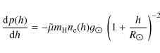
together with the equation of state in Eq. (1) gives the pressure stratification of the solar atmosphere. Here
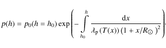
Here h0 denotes the height of the upper chromosphere - transition-region boundary and
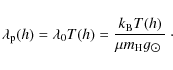
If the near-isothermal approximation (
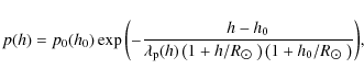
where the term
For a non-isothermal atmosphere, the following analytical approximation is applicable (Aschwanden & Schrijver 2002)

where the correction factor
Since the magnetic field usually dominates the force balance in the solar corona, it can be safely assumed that the cross-field transportation effects are negligible and the frozen-in and force-free approximations hold well in this environment. Hydrostatic balance along a given magnetic field line (loop strand; Martens 2009) can then be expressed in terms of the pressure and temperature dependence p = p(s), T = T(s), where s is the position along the field line, measured upwards from the photospheric footpoint s = 0 to the highest position on the field line (apex) s1. The correspondence between p(s) and p(h) is given by the field line geometry, i.e., the mapping
![]() .
.
The energy balance along a magnetic field line is determined by the balance of energy sources and sinks. In the stationary case it is given by the equilibrium between radiative losses ![]() ,
heating sources
,
heating sources ![]() ,
and the divergence of thermal conductive flux
,
and the divergence of thermal conductive flux
![]() ,
which can act both as a source or as a sink, depending on the temperature structure. The equation of energy balance in the stationary case is
,
which can act both as a source or as a sink, depending on the temperature structure. The equation of energy balance in the stationary case is
For the purposes of this study, we assume a simple one-piece power-law radiative-loss function
where
The form of the volumetric heating function ![]() is still unknown. It depends critically on the assumed physical heating mechanism(s). Here we make use of the parameterized form of the heating function introduced by Serio et al. (1981) and implemented by Aschwanden & Schrijver (2002) as
is still unknown. It depends critically on the assumed physical heating mechanism(s). Here we make use of the parameterized form of the heating function introduced by Serio et al. (1981) and implemented by Aschwanden & Schrijver (2002) as
This type of the heating function has two parameters:
Thermal conductive flux ![]() at position s along a given magnetic field line is given by (Spitzer 1962)
at position s along a given magnetic field line is given by (Spitzer 1962)
where
Further assumptions about the thermal conduction profile along a magnetic field line are
which mean that the magnetic field line is thermally isolated and its temperature profile T(s) is monotonic and has extrema only at both the footpoint and apex. These assumptions are necessary for integrating the temperature profile in both the temperature and spatial domains. In terms of a coronal loop, the assumptions given by Eqs. (11), (12) and (13) translates into a temperature maximum at the loop apex and a temperature minimum at the loop footpoint. The monotonical increase in temperature from footpoint to apex is ensured by the assumption in Eq. (13). The assumption in Eq. (11) means that the thermal conduction from the coronal loop into the chromosphere is negligible, i.e., the loop does not contribute to the heating of the underlying chromosphere. Equation (12) is the necessary, although not sufficient condition for loop symmetry. For the purposes of this paper, a geometrically symmetrical coronal loop of half-length L=s1 heated equivalently at both footpoints will be assumed. The loop is treated as a slender fluxtube along the chosen magnetic field line, which defines the loop geometry, i.e., the loop is represented by a one-dimensional loop strand (Martens 2009). The effect of the varying loop cross-section is neglected. This question is discussed later in Sect. 3.5.
2.2 Derivation of the scaling laws
Equation (7) can be integrated to obtain analytical formulae describing coronal loops. The assumptions (11), (12), and (13) allow us to integrate from the footpoint s0 to the loop apex s1 = L in both the temperature and geometrical domains. The derivation here proceeds in a way analogous to Priest (1982).
First we rewrite the pressure stratification of the solar atmosphere given by Eq. (5) or Eq. (6) in terms of the loop coordinate s and simplify it to the following form, which is equivalent to Eq. (9):
where
In the one-dimensional form of Eq. (7), the divergence operator
![]() .
changes to
.
changes to
![]() .
We multiply this equation by the factor
.
We multiply this equation by the factor
![]() ,
then substitute into this equation the Eqs. (8), (9) and (10), and then substitute the electron density
,
then substitute into this equation the Eqs. (8), (9) and (10), and then substitute the electron density ![]() by pressure according to Eqs. (1) and (14) to obtain
by pressure according to Eqs. (1) and (14) to obtain
Direct integration of this equation over the temperature range from the apex (coronal) temperature T1 to the lower transition-region temperature T0 is impossible, since the pressure scale-length
where
In the case of a typical coronal loop,
![]() .
If
.
If
![]() ,
then all terms containing T0 can be neglected. In the case of
,
then all terms containing T0 can be neglected. In the case of
![]() ,
the (coronal) loop apex temperature T1 would be strongly coupled to the temperature of the chromosphere. In the following,
,
the (coronal) loop apex temperature T1 would be strongly coupled to the temperature of the chromosphere. In the following,
![]() will always be assumed. Neglecting T0 immediately results in the following expression for the base pressure
will always be assumed. Neglecting T0 immediately results in the following expression for the base pressure
To obtain a second relation describing the coronal loop, Eq. (15) is integrated again from T1 to a temperature T',
where
will be used. Dividing the Eq. (18) by
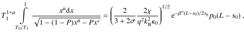
where the expressions
The value of T0 with respect to T1 can again be neglected. The integral function
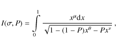
which exists only if
![\begin{figure}
\par\includegraphics[width=7.5cm,clip]{10899f1a.eps}
\includegraphics[width=7.5cm,clip]{10899f1b.eps}
\end{figure}](/articles/aa/full_html/2009/30/aa10899-08/img96.png) |
Figure 1:
Top: the
|
| Open with DEXTER | |
The condition ![]() results in formal bounding for the heating scale-height:
results in formal bounding for the heating scale-height:
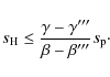
The shape of the
If the set of variables (L0,
![]() ,
,
![]() ), where
L0 = L-s0 is considered to be independent and T1 and p0 to be dependent variables, the scaling laws (17) and (20) can be easily rewritten to obtain the following expressions for T1 and p0:
), where
L0 = L-s0 is considered to be independent and T1 and p0 to be dependent variables, the scaling laws (17) and (20) can be easily rewritten to obtain the following expressions for T1 and p0:

Alternatively, the scaling laws can be written for the choice of
while the scaling law expressions S1 and S2 in our version (DDKK) take the form
| |
= |  |
(28) |
| = | (29) |
From Eq. (26), it is clear that the dependency of base pressure p0 on the apex temperature T1 is modified by the presence of the radiative-loss function parameter
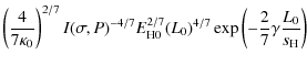
Equation (22) can be used to obtain
where
Table 1: Best-fit model coefficients in scaling laws expressions (32) and (31).
This form of the scaling laws for coronal loops is only a formal one, and for the completion one needs to determine the values of P, P', ![]() ,
,
![]() ,
,
![]() ,
and
,
and ![]() .
Unfortunately, without directly assuming the function T(s), their values cannot be determined analytically. Aschwanden & Schrijver (2002) found good analytical approximations of the function T(s) that depend on the geometrical properties of the loop, i.e., values of L and
.
Unfortunately, without directly assuming the function T(s), their values cannot be determined analytically. Aschwanden & Schrijver (2002) found good analytical approximations of the function T(s) that depend on the geometrical properties of the loop, i.e., values of L and ![]() ,
and also the apex temperature T1 (cf. their Eqs. (19)-(21) and Table 1). This means that the values of P, P',
,
and also the apex temperature T1 (cf. their Eqs. (19)-(21) and Table 1). This means that the values of P, P', ![]() ,
,
![]() ,
,
![]() ,
and
,
and ![]() can depend on the loop parameters L,
can depend on the loop parameters L, ![]() ,
and T1, i.e., they can change from loop to loop.
,
and T1, i.e., they can change from loop to loop.
At this point an adequate approximation is required. The simplest assumption that can be made is that these parameters are constants for the entire ranges of L and ![]() ,
while they (obviously) must change with the apex temperature T1. In other words, we assume that the temperature profile does not change much with L and
,
while they (obviously) must change with the apex temperature T1. In other words, we assume that the temperature profile does not change much with L and ![]() .
For this assumption, one can expect that the value of P will be close to unity, since P must approach unity for low
.
For this assumption, one can expect that the value of P will be close to unity, since P must approach unity for low
![]() values and shorter L, where the scaling laws of Rosner et al. (1978) hold.
To find the values of P, P',
values and shorter L, where the scaling laws of Rosner et al. (1978) hold.
To find the values of P, P', ![]() ,
,
![]() ,
,
![]() ,
and
,
and ![]() a numerical method for solving Eq. (7) with the appropriate boundary conditions must be invoked. The values of P, P',
a numerical method for solving Eq. (7) with the appropriate boundary conditions must be invoked. The values of P, P', ![]() ,
,
![]() ,
,
![]() ,
and
,
and ![]() can then be determined by direct fitting of the scaling laws (26) and (27) to the results of numerical simulations, for the assumption that
can then be determined by direct fitting of the scaling laws (26) and (27) to the results of numerical simulations, for the assumption that ![]() is the pressure scale-length corresponding to the apex temperature T1.
is the pressure scale-length corresponding to the apex temperature T1.
![\begin{figure}
\par\includegraphics[width=7.5cm,clip]{10899f2a.eps}\par\includegraphics[width=7.5cm,clip]{10899f2b.eps}
\end{figure}](/articles/aa/full_html/2009/30/aa10899-08/img126.png) |
Figure 2:
Scaling law for the base pressure p0 (Eqs. (26) and (31)) and base heating rate (Eqs. (27) and (32)) as a functions of L, |
| Open with DEXTER | |
To do this, we used the numeric code developed by Aschwanden & Schrijver (2002), which is part of the hydro package of the SolarSoft environment (Freeland & Handy 1998), running as a layer on top of the Interactive Data Language (IDL). The code enables one to choose from several implemented radiative-loss functions and then calculate solutions to Eq. (7). The chosen values of T0 and T1 together with Eqs. (11) and (12) represent the boundary conditions of a given loop. A fixed choice of T1 removes the difficulty of ![]() being a function of apex temperature. The value of s0 is determined by the height of the chromosphere together with the assumed loop geometry. We used the values of h0 = 1.3 Mm and
being a function of apex temperature. The value of s0 is determined by the height of the chromosphere together with the assumed loop geometry. We used the values of h0 = 1.3 Mm and
![]() K for the upper chromosphere, and L and
K for the upper chromosphere, and L and ![]() acted as independent variables. The code returns the values of
acted as independent variables. The code returns the values of
![]() and p0. Assuming a semi-circular loop geometry and executing the code multiple times for different choices of L and
and p0. Assuming a semi-circular loop geometry and executing the code multiple times for different choices of L and ![]() ,
we constructed a numerical grid of
,
we constructed a numerical grid of
![]() and p0 as functions of L and
and p0 as functions of L and ![]() .
The values of P, P',
.
The values of P, P', ![]() ,
,
![]() ,
,
![]() ,
and
,
and ![]() were then determined by the Levenberg-Marquardt method (Marquardt 1963), which minimizes the difference between the grid of numerical models and the scaling laws given by Eqs. (26) and (27) together with Eqs. (31) and (32). We indicate the parameter values for the choice of
were then determined by the Levenberg-Marquardt method (Marquardt 1963), which minimizes the difference between the grid of numerical models and the scaling laws given by Eqs. (26) and (27) together with Eqs. (31) and (32). We indicate the parameter values for the choice of
![]() ,
,
![]() Wm3 K1/2 (Kuin & Martens 1982), and 4 Mm
Wm3 K1/2 (Kuin & Martens 1982), and 4 Mm
![]() Mm, which is the same parameter space used by Aschwanden & Schrijver (2002). Since the computed numerical values of p0 and
Mm, which is the same parameter space used by Aschwanden & Schrijver (2002). Since the computed numerical values of p0 and
![]() span two and four orders of magnitude, respectively, the minimization was performed in logarithmic space. The results are summarized in Table 1.
span two and four orders of magnitude, respectively, the minimization was performed in logarithmic space. The results are summarized in Table 1.
For
![]() ,
the points in parameter space were excluded from the fitting procedure, because the numerical code often failed to converge here. The fitting accuracy of scaling laws is
,
the points in parameter space were excluded from the fitting procedure, because the numerical code often failed to converge here. The fitting accuracy of scaling laws is ![]() 40% for
40% for
![]() and
and ![]() 15% for p0. The accuracy is higher for lower
15% for p0. The accuracy is higher for lower
![]() values and rapidly decreased towards the
values and rapidly decreased towards the
![]() boundary. This is because for higher
boundary. This is because for higher
![]() values, the function T(s) changes rapidly (cf. Fig. 9 of Aschwanden & Schrijver 2002). The accuracy of the numerical solutions is less than 2%.
values, the function T(s) changes rapidly (cf. Fig. 9 of Aschwanden & Schrijver 2002). The accuracy of the numerical solutions is less than 2%.
The resulting dependency of p0 and
![]() on L,
on L, ![]() ,
and T1 is plotted in Fig. 2. In Fig. 3, the scaling laws are compared with numerical solutions and previously derived scaling laws of Rosner et al. (1978), Serio et al. (1981) and Aschwanden & Schrijver (2002). These plots are compiled in the same way as Figs. 4-6 of Aschwanden & Schrijver (2002) to facilitate direct visual comparison.
,
and T1 is plotted in Fig. 2. In Fig. 3, the scaling laws are compared with numerical solutions and previously derived scaling laws of Rosner et al. (1978), Serio et al. (1981) and Aschwanden & Schrijver (2002). These plots are compiled in the same way as Figs. 4-6 of Aschwanden & Schrijver (2002) to facilitate direct visual comparison.
![\begin{figure}
\par\includegraphics[width=12cm,clip]{aa10899-fig3.eps}
\end{figure}](/articles/aa/full_html/2009/30/aa10899-08/img132.png) |
Figure 3: Comparison of ``DDKK'' scaling laws (Eqs. (26), (27) together with Eqs. (31) and (32)) with the numerical solutions ( top row) and previously derived scaling laws of Rosner et al. (1978, second row), Serio et al. (1981, third row), and Aschwanden & Schrijver (2002, bottom row). Average ratios and standard deviations are given in each figure for each temperature separately. |
| Open with DEXTER | |
![\begin{figure}
\par\includegraphics[width=12cm,clip]{aa10899-fig4.eps}
\end{figure}](/articles/aa/full_html/2009/30/aa10899-08/img133.png) |
Figure 4:
Comparison of the numerical results for the base pressure
|
| Open with DEXTER | |
![\begin{figure}
\par\includegraphics[origin=rb,width=12cm,clip]{aa10899-fig5.eps}
\end{figure}](/articles/aa/full_html/2009/30/aa10899-08/img134.png) |
Figure 5:
Comparison of the numerical results for the base pressure p0 and base heating rate
|
| Open with DEXTER | |
![\begin{figure}
\par\includegraphics[width=12cm,clip]{aa10899-fig6.eps}
\end{figure}](/articles/aa/full_html/2009/30/aa10899-08/img135.png) |
Figure 6:
Same as in Fig. 5, but for the two radiative-loss functions
|
| Open with DEXTER | |
Slightly higher accuracy can be achieved by relaxing the assumption that ![]() ,
,
![]() ,
,
![]() ,
and
,
and ![]() are constants. If these parameters are allowed to vary slightly with L and
are constants. If these parameters are allowed to vary slightly with L and ![]() ,
the scaling law expressions in Eqs. (31) and (32) can be expanded into Taylor series. Neglecting terms higher than linear leads to
,
the scaling law expressions in Eqs. (31) and (32) can be expanded into Taylor series. Neglecting terms higher than linear leads to
where the expressions
3 Discussion
3.1 Hydrostatic scale-height
We note that the pressure scale-length ![]() is not equal to the pressure scale-height
is not equal to the pressure scale-height
![]() .
The pressure scale-length
.
The pressure scale-length ![]() is defined as the distance along the loop between points of pressure
p(s0) = p0 and
is defined as the distance along the loop between points of pressure
p(s0) = p0 and
![]() .
In contrast, pressure scale-height
.
In contrast, pressure scale-height
![]() is the vertical distance between the points s0, corresponding to height h0, and
is the vertical distance between the points s0, corresponding to height h0, and
![]() ,
corresponding to height
,
corresponding to height
![]() .
Since for a given loop geometry, the relation h = h(s) and the inverse relation s = s(h) is known, using the Eqs. (6) and (14), we can write approximately
.
Since for a given loop geometry, the relation h = h(s) and the inverse relation s = s(h) is known, using the Eqs. (6) and (14), we can write approximately

With the knowledge of the loop apex height h1, we can estimate

This equation was used in constructing the grid of numerical models in Sect. 2.2 for the assumption of semi-circular loop geometry.
3.2 Elliptical loops - a case study
In this section we perform a case study of the importance of different loop geometries on the resulting distributions of base pressure p0 and volumetric heating rate
![]() as functions of (L,
as functions of (L, ![]() ,
T1). The effects of varying loop geometry on hydrostatic loop solutions has not been studied previously the literature. Any possible effects on the resulting emission models were neglected (e.g., Schrijver et al. 2004).
,
T1). The effects of varying loop geometry on hydrostatic loop solutions has not been studied previously the literature. Any possible effects on the resulting emission models were neglected (e.g., Schrijver et al. 2004).
We computed a grid of numerical models identical to those in Sect. 2.2, but for loops of semi-elliptical shape. The semi-major to semi-minor axis ratio of these loops was chosen to equal 2, which corresponds to an eccentricity of ![]() .
In the first case, the semi-elliptical loops are oriented in portrait form, i.e., the photospheric footpoint baseline of the semi-elliptical loop is about a factor of 1.541 shorter than the photospheric footpoint baseline of the semi-circular loop with the same half-length L, while the apex is located 1.298-times higher. In the second studied case, the semi-elliptical loops are oriented landscape, i.e., the photospheric footpoint baseline of a such semi-elliptical loop is 1.298-times longer than the baseline of the semi-circular loop with the same half-length, while the apex is located
.
In the first case, the semi-elliptical loops are oriented in portrait form, i.e., the photospheric footpoint baseline of the semi-elliptical loop is about a factor of 1.541 shorter than the photospheric footpoint baseline of the semi-circular loop with the same half-length L, while the apex is located 1.298-times higher. In the second studied case, the semi-elliptical loops are oriented landscape, i.e., the photospheric footpoint baseline of a such semi-elliptical loop is 1.298-times longer than the baseline of the semi-circular loop with the same half-length, while the apex is located
![]() -times lower.
-times lower.
For the purpose of constructing the grid of numerical models, we modified the
![]() and
and
![]() routines of the hydro package by changing the employed h = h(s) function, which is for semi-elliptical loops given by the elliptic integral of the second kind, together with the component of gravitational force acting along the loop. We computed the grid of numerical models for four apex temperatures T1 = 1, 3, 5, and 10 MK. Unfortunately, we found that the numerical grid for the latest apex temperature was impossible to construct, because we encountered serious problems related to the spatial distribution of points s along loops. The problem appears for the entire range of recommended spatial distribution parameters (Aschwanden, private communication) and is left unresolved. However, computations for the first three apex temperatures were not affected by this problem. The results for the base heating rate
routines of the hydro package by changing the employed h = h(s) function, which is for semi-elliptical loops given by the elliptic integral of the second kind, together with the component of gravitational force acting along the loop. We computed the grid of numerical models for four apex temperatures T1 = 1, 3, 5, and 10 MK. Unfortunately, we found that the numerical grid for the latest apex temperature was impossible to construct, because we encountered serious problems related to the spatial distribution of points s along loops. The problem appears for the entire range of recommended spatial distribution parameters (Aschwanden, private communication) and is left unresolved. However, computations for the first three apex temperatures were not affected by this problem. The results for the base heating rate
![]() for these apex temperatures are displayed in Fig. 4. Taking into account that the error in the numerical simulations is less than 2%, we conclude that the effect of elliptical loop geometry is
for these apex temperatures are displayed in Fig. 4. Taking into account that the error in the numerical simulations is less than 2%, we conclude that the effect of elliptical loop geometry is ![]() 13% for the base heating rate
13% for the base heating rate
![]() for loops with
for loops with
![]() .
We note that because of Eq. (17), the relative changes in the base pressure p0 are expected to scale as the square root of the changes in the base heating rate
.
We note that because of Eq. (17), the relative changes in the base pressure p0 are expected to scale as the square root of the changes in the base heating rate
![]() .
Thus, the semi-elliptical loop geometry causes less than a
.
Thus, the semi-elliptical loop geometry causes less than a ![]() 6% difference in the base pressure p0.
6% difference in the base pressure p0.
The total changes
![]() in the radiative output of a loop due to the different loop geometry then scale as
in the radiative output of a loop due to the different loop geometry then scale as
We are unable to study the effects of elliptical loop geometry for higher values of the
3.3 Effect of radiative-loss function
We now study the effects of different radiative-loss functions on the density and temperature structure of the coronal loops. On the one hand, Eq. (26) together with Eq. (31) show the explicit dependence of the base pressure on the parameters ![]() and
and ![]() of the radiative-loss function (8). If we assume two different radiative-loss functions,
of the radiative-loss function (8). If we assume two different radiative-loss functions,
![]() and
and
![]() ,
we obtain the following expression for the ratio of the resulting base pressures
,
we obtain the following expression for the ratio of the resulting base pressures
 |
(37) |
where P1 and P2 can in general be different values for different radiative-loss functions. Similarly, the ratio of the resulting base heating rates
On the other hand, Eqs. (27) and (32) suggest that the volumetric base heating rate
![]() does not depend on
does not depend on ![]() ,
and depends only weakly on
,
and depends only weakly on ![]() through the
through the
![]() function. This result is confusing, since changes in total radiative output could in general require adjustments to the total energy input so that the assumed energy balance given by Eq. (7) is kept throughout the loop, even if the heating scale-length remains fixed, i.e., the volumetric heating rate
function. This result is confusing, since changes in total radiative output could in general require adjustments to the total energy input so that the assumed energy balance given by Eq. (7) is kept throughout the loop, even if the heating scale-length remains fixed, i.e., the volumetric heating rate
![]() could in general be dependent on
could in general be dependent on ![]() and
and ![]() .
.
To study this in more detail, we constructed a grid of numerical models using the radiative-loss functions
![]() and
and
![]() with
with
![]() Wm3,
Wm3,
![]() and
and
![]() Wm3 K2/3,
Wm3 K2/3,
![]() ,
which are the last two parts of the Rosner et al. (1978, Appendix A therein) analytical fit to the radiative-loss function of Raymond & Smith (1977). The first approximation is valid within the temperature range 105.75 K
< T < 106.3 K, and the second is valid for 106.3 K
< T < 107 K. We thus construct the grid of numerical models using the radiative-loss function
,
which are the last two parts of the Rosner et al. (1978, Appendix A therein) analytical fit to the radiative-loss function of Raymond & Smith (1977). The first approximation is valid within the temperature range 105.75 K
< T < 106.3 K, and the second is valid for 106.3 K
< T < 107 K. We thus construct the grid of numerical models using the radiative-loss function
![]() for the apex temperature T1 = 1 MK and the second radiative-loss function
for the apex temperature T1 = 1 MK and the second radiative-loss function
![]() for the apex temperatures T1 = 3 and 5 MK. Considering P = 1, the estimated values of p0 with respect to the values of
for the apex temperatures T1 = 3 and 5 MK. Considering P = 1, the estimated values of p0 with respect to the values of
![]() are
are
for the cases of T1 = 1, 3, and 5 MK, respectively. The estimated ratios of base heating rates for these three temperatures are 1.330, 0.919, and 0.919.
The results of numerical simulations using the two radiative-loss functions
![]() and
and
![]() are depicted in Figs. 5 and 6. It can be seen that for the case of
are depicted in Figs. 5 and 6. It can be seen that for the case of
![]() ,
the pressures
,
the pressures
![]() are close to their estimated values given by Eq. (39), while for
are close to their estimated values given by Eq. (39), while for
![]() ,
which deviates more significantly from the case
,
which deviates more significantly from the case
![]() ,
the results for
,
the results for
![]() are slightly further from the expected value. In all cases, the differences from the expected values given by Eq. (39) increases with increasing
are slightly further from the expected value. In all cases, the differences from the expected values given by Eq. (39) increases with increasing
![]() ratio.
ratio.
The values of the ratios
![]() and
and
![]() are wide-ranging, making the expected ratio values only a rough estimate. There are large deviations from the expected value for both strongly non-uniform heated loops (
are wide-ranging, making the expected ratio values only a rough estimate. There are large deviations from the expected value for both strongly non-uniform heated loops (
![]() )
and large loops (
)
and large loops (
![]() Mm). The ratio of base heating rates for the large loops approaches unity for all three studied apex temperatures.
Mm). The ratio of base heating rates for the large loops approaches unity for all three studied apex temperatures.
The discrepancies between results of numerical models and the expected values can be explained only in terms of the dependence of the T(s) function on the assumed radiative-loss function. For the fixed values of T1, L and ![]() ,
any change in the T(s) function will result in adjustments to the parameters P, P',
,
any change in the T(s) function will result in adjustments to the parameters P, P', ![]() ,
,
![]() ,
,
![]() ,
,
![]() and then implicitly in p0 and
and then implicitly in p0 and
![]() .
It can then be expected that the discrepancies will be in general larger for the heating rate ratios than for the base pressure ratios, because
.
It can then be expected that the discrepancies will be in general larger for the heating rate ratios than for the base pressure ratios, because
![]() ,
,
![]() (Table 1). However, the exact dependence of the T(s) function on assumed parameters of the radiative-loss function is not known except for the cases of uniform pressure and heating rate (Kuin & Martens 1982) and uniform pressure and heating explicitly dependent on temperature (Martens 2009). The reconstruction of the temperature profile from Eq. (18) is difficult because of the unknown dependence of
(Table 1). However, the exact dependence of the T(s) function on assumed parameters of the radiative-loss function is not known except for the cases of uniform pressure and heating rate (Kuin & Martens 1982) and uniform pressure and heating explicitly dependent on temperature (Martens 2009). The reconstruction of the temperature profile from Eq. (18) is difficult because of the unknown dependence of ![]() and
and ![]() on T'. We are thus left with direct construction of grids of numerical models in evaluating the effect of the radiative-loss function on the resulting distributions of p0 and
on T'. We are thus left with direct construction of grids of numerical models in evaluating the effect of the radiative-loss function on the resulting distributions of p0 and
![]() .
.
3.4 Scaling law for apex temperature
In this section we return to Eq. (24), which gives the apex temperature as a function of
![]() ,
and
,
and
![]() .
The choice of
.
The choice of
![]() ,
and
,
and
![]() as independent parameters is more natural from the perspective of modeling coronal emission in EUV and soft X-ray (e.g., Schrijver et al. 2004), since the coronal emission in the EUV or soft X-ray filter is given by the product of
as independent parameters is more natural from the perspective of modeling coronal emission in EUV and soft X-ray (e.g., Schrijver et al. 2004), since the coronal emission in the EUV or soft X-ray filter is given by the product of
![]() and the filter response (Mok et al. 2005, and references therein), the latter being a function of both the temperature and electron density.
and the filter response (Mok et al. 2005, and references therein), the latter being a function of both the temperature and electron density.
The values of
![]() ,
and
,
and ![]() appearing in Eqs. (24) and (25) together with the values of
appearing in Eqs. (24) and (25) together with the values of ![]() and
and ![]() were reconstructed from the values of
were reconstructed from the values of
![]() ,
and
,
and ![]() and are listed in Table 2.
and are listed in Table 2.
Table 2: Coefficients in scaling laws (24) and (25) reconstructed from values in Table 1.
Using the numerically obtained values of
![]() ,
it is possible to reconstruct the apex temperature T1 as function of
,
it is possible to reconstruct the apex temperature T1 as function of
![]() ,
and
,
and
![]() .
The results are shown in Fig. 7, which suggests that the resulting apex temperatures T1 are within 20% of their expected values.
.
The results are shown in Fig. 7, which suggests that the resulting apex temperatures T1 are within 20% of their expected values.
We note that the expression
![]() is negative for all studied apex temperatures. The inequality sign in the condition (23) must then be reversed, so that it is always satisfied.
is negative for all studied apex temperatures. The inequality sign in the condition (23) must then be reversed, so that it is always satisfied.
![\begin{figure}
\par\includegraphics[width=8.8cm,clip]{10899f7.eps}
\end{figure}](/articles/aa/full_html/2009/30/aa10899-08/img182.png) |
Figure 7:
Scaling law for the apex temperature T1 as function of L, |
| Open with DEXTER | |
3.5 Loops with expanding cross-section
We now focus our attention on the effect of the expanding cross-section of the loop. We examine in particular the concept of a loop as an expanding magnetic fluxtube. We utilized the geometry of expanding loops with a buried dipole of Aschwanden & Schrijver (2002), which generalizes the expanding loop model of Vesecky et al. (1979) for an arbitrary large range of loop expansion factors ![]() .
The loop expansion factor is defined to be
.
The loop expansion factor is defined to be
![]() ,
where A1 and A0 are the apex and photospherical cross-sections of the loop, respectively. The geometrical model of the expanding loop of Aschwanden & Schrijver (2002) employs the semi-circular geometry in an expanding toroidal shell around the central, semi-circular magnetic field line or loop strand. The central vertical cut through the loop containing the central magnetic field line is depicted in Fig. 3.14 right panel of Aschwanden (2004).
,
where A1 and A0 are the apex and photospherical cross-sections of the loop, respectively. The geometrical model of the expanding loop of Aschwanden & Schrijver (2002) employs the semi-circular geometry in an expanding toroidal shell around the central, semi-circular magnetic field line or loop strand. The central vertical cut through the loop containing the central magnetic field line is depicted in Fig. 3.14 right panel of Aschwanden (2004).
Previous authors (Aschwanden & Schrijver 2002; Martens 2009; Vesecky et al. 1979) claimed that the effect of expanding loop cross-section on the temperature profile T(s) is small. However, after considering the expanding geometry of Aschwanden & Schrijver (2002), it is clear that the inward (lowermost) and outward (topmost) field lines or loop strands of the expanding fluxtube have different lengths, and because of Eqs. (24) and (25) they must have different apex temperatures and base pressures; i.e.,
![]() ,
,
![]() .
This means that the emission from these two field lines observed in EUV or X-ray filters must differ. To study this, we computed the ratio of the inward loop strand to the outward loop strand apex emissions in two TRACE filters, 171 and 195 Å.
.
This means that the emission from these two field lines observed in EUV or X-ray filters must differ. To study this, we computed the ratio of the inward loop strand to the outward loop strand apex emissions in two TRACE filters, 171 and 195 Å.
The length
![]() and
and
![]() of the coronal portion of the inward and outward loop strands are given by
of the coronal portion of the inward and outward loop strands are given by
where
where
We assume that L0 is the length of the coronal portion of the central strand and the heating parameters
![]() and
and ![]() do not change for the entire loop. The computation of the emission ratio proceeds as follows. First, we choose the apex temperature of the central loop strand
do not change for the entire loop. The computation of the emission ratio proceeds as follows. First, we choose the apex temperature of the central loop strand
![]() from the interval
from the interval ![]() MK, 1.5 MK
MK, 1.5 MK![]() .
Equation (27) then gives the base heating rate
.
Equation (27) then gives the base heating rate
![]() for the chosen central strand apex temperature. The lengths
for the chosen central strand apex temperature. The lengths
![]() and
and
![]() are then computed using Eqs. (40). These values were inserted into Eqs. (24) and (25), which provide the apex temperatures
are then computed using Eqs. (40). These values were inserted into Eqs. (24) and (25), which provide the apex temperatures
![]() ,
,
![]() and the base pressures
and the base pressures
![]() and
and
![]() as functions of
as functions of
![]() ,
and
,
and ![]() .
The apex densities
.
The apex densities
![]() and
and
![]() were computed using Eqs. (14), (36), (4), and (1). The computed values of
were computed using Eqs. (14), (36), (4), and (1). The computed values of
![]() ,
,
![]() ,
,
![]() ,
and
,
and
![]() were then used together with the TRACE filter response (Mok et al. 2005) for 171 and 195 Å filters to obtain the emissions in the corresponding filter.
were then used together with the TRACE filter response (Mok et al. 2005) for 171 and 195 Å filters to obtain the emissions in the corresponding filter.
![\begin{figure}
\par\includegraphics[width=12cm,clip]{aa10899-fig8.eps}
\end{figure}](/articles/aa/full_html/2009/30/aa10899-08/img218.png) |
Figure 8:
Computed ratios of emission at apexes of the inward (i) and outward (o) loop strands as function of |
| Open with DEXTER | |
The emission ratio is expected to increase with increasing ![]() ,
A0, and decreasing L0, because of the increasing difference between
,
A0, and decreasing L0, because of the increasing difference between
![]() and
and
![]() .
We also note that if the apex temperature
.
We also note that if the apex temperature
![]() of the central strand is close to the temperature for which the filter response reaches its maximum (
of the central strand is close to the temperature for which the filter response reaches its maximum (![]() 1 MK for the 171 Å filter, and
1 MK for the 171 Å filter, and ![]() 1.5 MK for the 195 Å filter), then the computed emission ratio should be close to unity; this is because the apex temperatures of the inward and outward strands
1.5 MK for the 195 Å filter), then the computed emission ratio should be close to unity; this is because the apex temperatures of the inward and outward strands
![]() and
and
![]() will correspond to roughly equal values of the filter response. The situation will be different for temperatures where the filter response is decreasing (
will correspond to roughly equal values of the filter response. The situation will be different for temperatures where the filter response is decreasing (
![]() MK for 171 Å filter) or increasing (
MK for 171 Å filter) or increasing (
![]() MK for 195 Å filter), where the difference between the
MK for 195 Å filter), where the difference between the
![]() and
and
![]() would increase the observed emission ratio.
would increase the observed emission ratio.
We present the results for the case of uniform heating (L = 40 Mm,
![]() Mm; Fig. 8 top row) and non-uniform heating (L = 40 Mm,
Mm; Fig. 8 top row) and non-uniform heating (L = 40 Mm,
![]() Mm; Fig. 8 bottom row). For both these cases, the ratio of the computed emission is too low to explain the observed narrowness of coronal loops (López Fuentes et al. 2006; Klimchuk 2000; Watko & Klimchuk 2000). The only case where the emission ratio could suffice to explain the observed narrowness of the coronal loops is the case of short (
Mm; Fig. 8 bottom row). For both these cases, the ratio of the computed emission is too low to explain the observed narrowness of coronal loops (López Fuentes et al. 2006; Klimchuk 2000; Watko & Klimchuk 2000). The only case where the emission ratio could suffice to explain the observed narrowness of the coronal loops is the case of short (
![]() Mm), uniformly heated loops, since the ratio reaches a factor of
Mm), uniformly heated loops, since the ratio reaches a factor of ![]() 5 or more for these loops. We thus conclude that in general the difference in lengths of the inward and outward loop strands cannot explain the observed spatial profile of coronal loops. For stationary, near-potential coronal loops obeying the scaling laws, the parameters of the heating function within a magnetic fluxtube with photospheric cross-sections corresponding to the TRACE resolution (1
5 or more for these loops. We thus conclude that in general the difference in lengths of the inward and outward loop strands cannot explain the observed spatial profile of coronal loops. For stationary, near-potential coronal loops obeying the scaling laws, the parameters of the heating function within a magnetic fluxtube with photospheric cross-sections corresponding to the TRACE resolution (1
![]() )
must vary rapidly to produce a coronal loop with the observed narrowness.
)
must vary rapidly to produce a coronal loop with the observed narrowness.
4 Conclusions
We have derived an analytical set of scaling laws between loop apex temperature T1, base pressure p0, base heating rate
![]() ,
loop half-length L, and heating scale length
,
loop half-length L, and heating scale length ![]() for geometrically symmetrical, non-uniformly heated, and gravitationally stratified one-dimensional loop strands that are thermally isolated with monotonically increasing temperature profile. For analytical treatability, the derivation of the scaling laws employed the mean-value theorem, which directly implied the need of fitting the analytical results to the numerical simulations under the assumption of constant mean-value parameters. This strict assumption in turn leads to moderate accuracy of the scaling laws with respect to the numerical simulations. Higher accuracy can be achieved only by employing Taylor expansion or additional empirical terms. The latter provides higher precision, and ensures that the scaling laws of Aschwanden & Schrijver (2002) are the most precise scaling laws existing to date, even though their empirical terms have no analytical background. However, the presence of d0 and e0 parameters is justified in terms of our parameter P' and the
for geometrically symmetrical, non-uniformly heated, and gravitationally stratified one-dimensional loop strands that are thermally isolated with monotonically increasing temperature profile. For analytical treatability, the derivation of the scaling laws employed the mean-value theorem, which directly implied the need of fitting the analytical results to the numerical simulations under the assumption of constant mean-value parameters. This strict assumption in turn leads to moderate accuracy of the scaling laws with respect to the numerical simulations. Higher accuracy can be achieved only by employing Taylor expansion or additional empirical terms. The latter provides higher precision, and ensures that the scaling laws of Aschwanden & Schrijver (2002) are the most precise scaling laws existing to date, even though their empirical terms have no analytical background. However, the presence of d0 and e0 parameters is justified in terms of our parameter P' and the
![]() function.
function.
We performed a case study of the semi-elliptical loop geometries. The difference in loop geometry results only in relatively small changes in p0 and
![]() ,
of the order of less than approximately 6% for p0 and about twice as much for
,
of the order of less than approximately 6% for p0 and about twice as much for
![]() .
The results are more sensitive to the parameters of the radiative-loss function. The base pressure p0 depends explicitly on both
.
The results are more sensitive to the parameters of the radiative-loss function. The base pressure p0 depends explicitly on both ![]() and
and ![]() ,
while the dependence of the base heating rate
,
while the dependence of the base heating rate
![]() on these parameters is apart from the presence of the
on these parameters is apart from the presence of the
![]() function by means of the temperature profile. However, the effect of radiative-loss function is non-negligible and thus a correct power-law approximation to the radiative-loss function must be taken before the scaling laws are applied, e.g., in forward modeling of coronal emission. It is interesting that the base heating rate
function by means of the temperature profile. However, the effect of radiative-loss function is non-negligible and thus a correct power-law approximation to the radiative-loss function must be taken before the scaling laws are applied, e.g., in forward modeling of coronal emission. It is interesting that the base heating rate
![]() for long, uniformly heated loops is almost independent of the details of the radiative-loss function.
for long, uniformly heated loops is almost independent of the details of the radiative-loss function.
The effect of an expanding loop cross-section on the resulting EUV emission in TRACE 171 Å and 195 Å filters was studied. We conclude that the different lengths of the inward and outward loop strand are insufficient to explain the spatial narrowness of coronal loops except for the case of small, uniformly heated loops, i.e., if the parameters of the heating function did not vary in space, both inward and outward loop strands would be visible in a given TRACE EUV filter.
Appendix A: Mean-value theorem
The mean-value theorem for integration (e.g., Bartsch 1977) states that for the integrable function f(x) and continuous function g(x),
![]() ,
there exists a number
,
there exists a number
![]() ,
for which the following relation holds:
,
for which the following relation holds:
We demonstrate the use of this theorem in evaluating the integral J defined by (cf. Eq. (15))
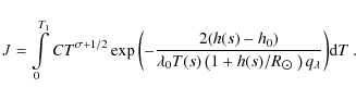
Here we must take into account that because of the assumptions presented in Eqs. (11), (12), and (13), the temperature profile T(s) monotonically increases, which means that there exists a unique and monotonic inverse function s = s(T). Similarly, due to the h = h(s) dependence, there exists a unique h = h(T) function.
Using the mean-value theorem it is clear that there exists some
![]() for which the integral (A.2) equals to
for which the integral (A.2) equals to
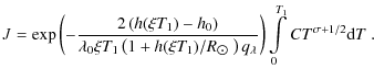
Since the function h(T) is monotonic, there must exist some
Thus the integral J equals to
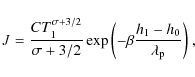
where
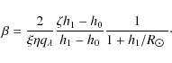
Equation (36) can be used to convert Eq. (A.6) into the final result
We note that the
Acknowledgements
The authors are thankful to the referee, P. Martens, for his comments that helped to clarify several issues in the manuscript. We are indebted to M. Aschwanden for incorporating the hydro package into the SolarSoft library, thus providing us with a powerful and versatile tool to study the equilibrium solutions for coronal loops. We are also thankful for helpful and lengthy discussions regarding the software. We would also like to extend our thanks to J. Klacka for helpful discussion regarding thefunction. This work was supported by Scientific Grant Agency, VEGA, Slovakia, Grant No. 1/0069/08, Grant IAA300030701 of the Grant Agency of the Academy of Sciences of the Czech Republic and ESA-PECS project No. 98030. J.D. also acknowledges the financial support of the Comenius University Grant No. 414/2008. The Solar and Heliospheric Observatory (SOHO) is a project of international cooperation between ESA and NASA. The Transition Region and Coronal Explorer (TRACE) is a mission of the Stanford-Lockheed Institute for Space Research, and part of the NASA Small Explorer program.
References
- Antiochos, S. K. 1979, ApJ, 232, L125 [NASA ADS] [CrossRef]
- Aschwanden, M. J. 2004, Physics of the Solar Corona: An Introduction (United Kingdom: Springer, PRAXIS, Chichester) (In the text)
- Aschwanden, M. J., & Schrijver, C. J. 2002, ApJ, 142, 269 [NASA ADS] [CrossRef]
- Aschwanden, M. J., & Tsiklauri, D. 2009, ApJ, submitted (In the text)
- Bartsch, H.-J. 1977, Mathematische Formeln (Germany: VEB Fachbuchverlag, Leipzig) (In the text)
- Chiuderi, C., Einaudi, G., & Torricelli-Ciamponi, G. 1981, A&A, 97, 27 [NASA ADS]
- Craig, I. J. D., McClymont, A. N., & Underwood, J. H. 1978, A&A, 70, 1 [NASA ADS]
- Craig, I. J. D., Robb, T. D. & Rollo, M. D. 1982, Sol. Phys., 76, 331 [NASA ADS] [CrossRef]
- Freeland, S. L., & Handy, B. N. 1998, Sol. Phys., 182, 497 [NASA ADS] [CrossRef] (In the text)
- Handy, B. N., Acton, L. W., Kankelborg, C. C., et al. 1999, Sol. Phys., 187, 229 [NASA ADS] [CrossRef] (In the text)
- Hood, A. W., & Priest, E. R. 1979, A&A, 77, 233 [NASA ADS]
- Hood, A. W., & Priest, E. R. 1980, A&A, 87, 126 [NASA ADS]
- Klimchuk, J. A. 2000, Sol. Phys., 193, 53 [NASA ADS] [CrossRef]
- Klimchuk, J. A. 2006, Sol. Phys., 234, 41 [NASA ADS] [CrossRef] (In the text)
- Kuin, N. P. M., & Martens, P. C. H. 1982, A&A, 108, L1 [NASA ADS]
- López Fuentes, M. C., Klimchuk, J. A., & Démoulin, P. 2006, ApJ, 639, 459 [NASA ADS] [CrossRef]
- Marquardt, D. W. 1963, J. Soc. Indust. Appl. Math., 11, 431 [CrossRef] (In the text)
- Martens, P. C. H. 2009, ApJ, submitted
- Martens, P. C. H., Kankelborg, C. C., & Berger, T. E. 2000, ApJ, 537, 471 [NASA ADS] [CrossRef]
- Mok, Y., Mikic, Z., Lionello, R., & Linker, J. A. 2005, ApJ, 621, 1098 [NASA ADS] [CrossRef] (In the text)
- Priest, E. R. 1982, Solar Magnetohydrodynamics (Holland: D. Reidel Publishing Company, Dordrecht) (In the text)
- Raymond, J. C., & Smith, B. W. 1977, ApJS, 35, 419 [NASA ADS] [CrossRef] (In the text)
- Rosner, R., Tucker, W. H., & Vaiana, G. S. 1978, ApJ, 220, 643 [NASA ADS] [CrossRef]
- Scherrer, P. H., Bogart, R. S., Bush, R. I., et al. 1995, Sol. Phys., 162, 129 [NASA ADS] [CrossRef] (In the text)
- Schrijver, C. J., Sandman, A. W., Aschwanden, M. J., & DeRosa, M. L. 2004, ApJ, 615, 512 [NASA ADS] [CrossRef] (In the text)
- Serio, S., Peres, G., Vaiana, G. S., et al. 1981, ApJ, 243, 288 [NASA ADS] [CrossRef]
- Spitzer, L. 1962, Physics of Fully Ionized Gases (New York: Interscience) (In the text)
- Tucker, W. H., & Koren, M. 1971, ApJ, 168, 283 [NASA ADS] [CrossRef] (In the text)
- Vesecky, J. F., Antiochos, S. K., & Underwood, J. H. 1979, ApJ, 233, 987 [NASA ADS] [CrossRef] (In the text)
- Watko, J. A., & Klimchuk, J. A. 2000, Sol. Phys., 193, 77 [NASA ADS] [CrossRef]
- Wragg, M. A., & Priest, E. R. 1981, Sol. Phys., 70, 293 [NASA ADS] [CrossRef]
All Tables
Table 1: Best-fit model coefficients in scaling laws expressions (32) and (31).
Table 2: Coefficients in scaling laws (24) and (25) reconstructed from values in Table 1.
All Figures
| |
Figure 1:
Top: the
|
| Open with DEXTER | |
| In the text | |
| |
Figure 2:
Scaling law for the base pressure p0 (Eqs. (26) and (31)) and base heating rate (Eqs. (27) and (32)) as a functions of L, |
| Open with DEXTER | |
| In the text | |
| |
Figure 3: Comparison of ``DDKK'' scaling laws (Eqs. (26), (27) together with Eqs. (31) and (32)) with the numerical solutions ( top row) and previously derived scaling laws of Rosner et al. (1978, second row), Serio et al. (1981, third row), and Aschwanden & Schrijver (2002, bottom row). Average ratios and standard deviations are given in each figure for each temperature separately. |
| Open with DEXTER | |
| In the text | |
| |
Figure 4:
Comparison of the numerical results for the base pressure
|
| Open with DEXTER | |
| In the text | |
| |
Figure 5:
Comparison of the numerical results for the base pressure p0 and base heating rate
|
| Open with DEXTER | |
| In the text | |
| |
Figure 6:
Same as in Fig. 5, but for the two radiative-loss functions
|
| Open with DEXTER | |
| In the text | |
| |
Figure 7:
Scaling law for the apex temperature T1 as function of L, |
| Open with DEXTER | |
| In the text | |
| |
Figure 8:
Computed ratios of emission at apexes of the inward (i) and outward (o) loop strands as function of |
| Open with DEXTER | |
| In the text | |
Copyright ESO 2009
Current usage metrics show cumulative count of Article Views (full-text article views including HTML views, PDF and ePub downloads, according to the available data) and Abstracts Views on Vision4Press platform.
Data correspond to usage on the plateform after 2015. The current usage metrics is available 48-96 hours after online publication and is updated daily on week days.
Initial download of the metrics may take a while.