| Issue |
A&A
Volume 495, Number 1, February III 2009
|
|
|---|---|---|
| Page(s) | 147 - 155 | |
| Section | Galactic structure, stellar clusters, and populations | |
| DOI | https://doi.org/10.1051/0004-6361/200809886 | |
| Published online | 30 January 2009 | |
No evidence of mass segregation in massive young clusters
J. Ascenso1,2 - J. Alves3 - M. T. V. T. Lago1,4
1 - Centro de Astrofísica da Universidade do Porto, Rua das
Estrelas, 4150-762 Porto, Portugal
2 - Harvard-Smithsonian Center
for Astrophysics, 60 Garden Street, Cambridge, MA 02138, USA
3 -
Calar Alto Observatory - Centro Astronómico Hispano-Alemán, C/
Jesús Durbán Remón 2-2, 04004 Almeria, Spain
4 - Departamento
de Matemática Aplicada da Faculdade de Ciências, Universidade do
Porto, Rua do Campo Alegre, 657,
4169-007 Porto, Portugal
Received 1 April 2008 / Accepted 17 November 2008
Abstract
Aims. We investigate the validity of the mass segregation indicators commonly used in analysing young stellar clusters.
Methods. We simulate observations by constructing synthetic seeing-limited images of a 1000 massive clusters (10
![]() )
with a standard IMF and a King-density distribution function.
)
with a standard IMF and a King-density distribution function.
Results. We find that commonly used indicators are highly sensitive to sample incompleteness in observational data and that radial completeness determinations do not provide satisfactory corrections, rendering the studies of radial properties highly uncertain. On the other hand, we find that, under certain conditions, the global completeness can be estimated accurately, allowing for the correction of the global luminosity and mass functions of the cluster.
Conclusions. We argue that there is currently no observational evidence of mass segregation in young compact clusters since there is no robust way to differentiate between true mass segregation and sample incompleteness effects. Caution should then be exercised when interpreting results from observations as evidence of mass segregation.
Key words: open clusters and associations: general - methods: statistical
1 Introduction
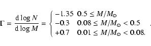
The issue of mass segregation in globular and open clusters has been discussed in the literature for over 20 years. Historically, the first indicator of mass segregation was simply that the brightest, most massive cluster members lay closest to the cluster core, whereas the faintest, lower-mass members fill the whole extent of the cluster area (McNamara & Sekiguchi 1986, and references therein). The mass segregation issue has since been complemented with specific properties that overall quantify the differences in the spatial distribution of high- and low-mass stars. The most commonly used for this effect are: (1) the radial dependence of the mass function (e.g., Schweizer 2004; Moitinho et al. 1997; Gouliermis et al. 2004; Stolte et al. 2006) or luminosity function (e.g., de Grijs et al. 2002; Jones & Stauffer 1991); (2) the radial differences in the ratio of high- to low-mass stars (e.g., Hillenbrand 1997); (3) the mean mass within some characteristic radius (e.g., Hillenbrand & Hartmann 1998; Sagar et al. 1988); and (4) the mean radius of the two distributions (e.g., de Grijs et al. 2002; Sagar et al. 1988) or the direct comparison of the cumulative radial density distribution for the two subsamples (e.g., McNamara & Sekiguchi 1986; Tadross 2005).
Even though almost all young clusters present one or more of these properties, several authors have shown that the timescale for dynamical relaxation is typically longer than the clusters' age (e.g., Bonnell & Davies 1998), implying that the observed mass segregation should not be dynamical in origin. Faster phenomena, such as violent relaxation (Binney & Tremaine 1987; Hillenbrand & Hartmann 1998) and the fact that the massive stars have shorter relaxation times (Hillenbrand & Hartmann 1998, and references therein) still do not seem to be sufficient for explaining the profusion of young clusters presenting these properties or the implicit degree of mass segregation. The alternative is a primordial origin, in which the distribution of massive stars in young clusters must reflect the initial conditions and the processes involved in cluster formation (e.g., Bonnell 2000).
![\begin{figure}
\par\includegraphics[width=14.5cm,clip]{09886fig01.eps}
\end{figure}](/articles/aa/full_html/2009/07/aa09886-08/img10.gif) |
Figure 1:
Left: Salpeter (1955) (
|
| Open with DEXTER | |
Conversely, some authors have indirectly shown that the way some
indicators are presented is not statistically accurate. For example,
Maíz Apellániz & Úbeda (2005) prove that a significant bias is introduced
when building the mass function in equal
![]() bins,
as is done in the literature. A statistical bias is also potentially
introduced when studying the radial properties of a cluster by
dividing the cluster area in fixed-width or constant-area annuli
rather than equal-number annuli, as each annulus will contain
different numbers of stars changing the statistical significance from
one annulus to the next.
bins,
as is done in the literature. A statistical bias is also potentially
introduced when studying the radial properties of a cluster by
dividing the cluster area in fixed-width or constant-area annuli
rather than equal-number annuli, as each annulus will contain
different numbers of stars changing the statistical significance from
one annulus to the next.
In this paper we propose to investigate the validity of a few
traditional mass segregation indicators using synthetic,
![]() -class clusters. We describe the biases that result directly
from the binning of the data and then explore the incompleteness in
observed samples and its consequences on the mass segregation
indicators.
-class clusters. We describe the biases that result directly
from the binning of the data and then explore the incompleteness in
observed samples and its consequences on the mass segregation
indicators.
The nomenclature used throughout the text is summarised as follows:
- True clusters: synthetic clusters
(Sect. 2.1).
- Observed* clusters: synthetic observations
(Sect. 2.2).
- Completeness tests: completeness
assessment obtained by adding artificial stars of increasing magnitude
to the cluster image in a grid. Derived completeness is defined as the
number of detected grid stars with measured magnitudes
 that
satisfy the condition
that
satisfy the condition
 ,
divided by the total
number of stars of magnitude
,
divided by the total
number of stars of magnitude
 in the input grid
(Sect. 4.1). This would be the assessment an
observer could do in real data.
in the input grid
(Sect. 4.1). This would be the assessment an
observer could do in real data.
- True completeness: completeness assessment obtained by direct comparison of the observed* and true clusters. Derived completeness is defined as the number of stars in the observed* cluster divided by the corresponding number of stars in the true cluster (Sect. 4.2). This assessment is only possible because we know the true composition of the cluster.
2 Simulations
2.1 Synthetic clusters
We created 1000 synthetic clusters, each containing
![]() stars (total mass of
stars (total mass of
![]() ). Each cluster member
was assigned a mass from a Salpeter (1955) (
). Each cluster member
was assigned a mass from a Salpeter (1955) (
![]() )
and Kroupa (2001) (
)
and Kroupa (2001) (
![]() )
IMF (Fig. 1, left):
)
IMF (Fig. 1, left):
The radial position (distance to the centre) of each artificial star was drawn randomly and independently of mass from a King (1962) radial surface density profile (Fig. 1, right):
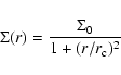
with a core radius
2.2 Synthetic observations
![\begin{figure}
\par\includegraphics[width=14.5cm,clip]{09886fig02.eps}
\end{figure}](/articles/aa/full_html/2009/07/aa09886-08/img23.gif) |
Figure 2: Seeing limited images of three simulated clusters. The brightness of the sources corresponds to the K-band. |
| Open with DEXTER | |
To investigate the impact of incompleteness due to crowding - a strong
limitation in most studies of mass segregation in real (massive)
clusters - we have used IRAF mkobject to build ``seeing
limited'' images of the synthetic clusters. The masses were
transformed into K-band luminosities using the mass-luminosity
relation from Ascenso et al. (2007) for a distance of 3 kpc and no
interstellar extinction. This configuration produced stars up to
magnitude 19. Since the Monte Carlo algorithm for the positions only
generates the r polar coordinates, a value for ![]() was assigned
to each r from a uniform random distribution between 0 and
was assigned
to each r from a uniform random distribution between 0 and
![]() .
Figure 2 shows three of the clusters
obtained in this way.
.
Figure 2 shows three of the clusters
obtained in this way.
These images were treated as actually observed clusters, in the sense
that they were subjected to a source extraction algorithm (IRAF daofind), PSF photometry (IRAF allstar), and cuts in
photometric errors to produce the final samples. These synthetic
observations were only sensitive to stars up to magnitude 16.5, with
only ![]() 29% of the original sources up to this magnitude being
detected. The 1000 catalogues produced in this way are hence
incomplete sub-samples of the original synthetic clusters. Since they
are meant to pose as real observations, we will hereafter refer to the
(incomplete) sub-samples as observed*, always maintaining the
asterisk to avoid confusion with actual observations that are not
presented here. The properties of the (complete) clusters originally
generated by the simulations will be labeled as ``true'', since
they refer to all the stars.
29% of the original sources up to this magnitude being
detected. The 1000 catalogues produced in this way are hence
incomplete sub-samples of the original synthetic clusters. Since they
are meant to pose as real observations, we will hereafter refer to the
(incomplete) sub-samples as observed*, always maintaining the
asterisk to avoid confusion with actual observations that are not
presented here. The properties of the (complete) clusters originally
generated by the simulations will be labeled as ``true'', since
they refer to all the stars.
3 Results
We tested the most commonly used mass segregation indicators on synthetic, non-segregated clusters to investigate how the way we approach observational data may influence our perception of mass segregation in massive clusters.
For each indicator we investigate: (1) the results expected for a non-segregated cluster; (2) the statistical effects of binning; and (3) the effects of incompleteness of the sample due to crowding. The first item is measured directly from the synthetic clusters and averaged over the whole set to produce the expected properties of a ``perfect cluster''. The second concerns the way the quantities are represented and how it may affect the analysis. The third is measured on the observed* clusters to explore in which ways the incompleteness of the observed samples due to crowding can mimic the effects of mass segregation.
We used the full width at half maximum of the stars in the simulated observations (5 pixels) as the (arbitrary) unit of length.
3.1 Slope vs. radius
The variation of the mass function (MF) with radius is already a
traditional diagnosis tool for mass segregation
(Bica & Bonatto 2005; de Grijs et al. 2002; Moitinho et al. 1997; Stolte et al. 2002,2005; Gouliermis et al. 2004; Bonatto & Bica 2005). In
a mass segregated cluster we expect to find an increase in the number
of massive stars with respect to the number of low-mass stars toward
the centre, which translates into a flattening of the mass function or
an increase of the high-mass end slope, hereafter referred simply as
slope or ![]() .
Conversely, in a non-segregated cluster we expect
the slope to be constant with radius.
.
Conversely, in a non-segregated cluster we expect
the slope to be constant with radius.
3.1.1 Binning effects
This section discusses the MF slope analysis performed on the original
![]() -star clusters.
-star clusters.
When investigating the radial dependence of the mass function we must
bin the data twice: first we divide the cluster area into concentric
annuli and then bin the masses of the objects in each annulus to
produce the mass function for that annulus. In order to keep the
statistical significance and avoid biases, these bins should be
defined such as to keep the number of stars per bin
constant. Historically, the radial bins are defined as fixed-width or
fixed-area annuli, whereas the mass bins are defined from the
histogram of
![]() ,
as constant
,
as constant
![]() bins, neither one keeping the number of stars per bin constant.
Instead, the radial bins should be defined as equal-number annuli, and
the mass function as a histogram with each bin containing the same
number of stars and divided by the resultant bin width
(Maíz Apellániz & Úbeda 2005).
bins, neither one keeping the number of stars per bin constant.
Instead, the radial bins should be defined as equal-number annuli, and
the mass function as a histogram with each bin containing the same
number of stars and divided by the resultant bin width
(Maíz Apellániz & Úbeda 2005).
![\begin{figure}
\par\includegraphics[width=14cm,clip]{09886fig03.eps}
\end{figure}](/articles/aa/full_html/2009/07/aa09886-08/img28.gif) |
Figure 3:
Mass function slope ( |
| Open with DEXTER | |
Figure 3 shows the variation of ![]() with
radius for the 1000 synthetic
with
radius for the 1000 synthetic
![]() -star clusters, calculated
with several combinations of radial and mass bins. The three panels to
the left have the masses appropriately binned, according to
Maíz Apellániz & Úbeda (2005), whereas the panels to the right are produced
using the more traditional mass functions from fixed
-star clusters, calculated
with several combinations of radial and mass bins. The three panels to
the left have the masses appropriately binned, according to
Maíz Apellániz & Úbeda (2005), whereas the panels to the right are produced
using the more traditional mass functions from fixed
![]() histograms of
histograms of
![]() .
In the
two top panels the radii are binned in annuli with equal number (100)
of stars, the middle panels have fixed-width (10 FWHM) radial annuli,
and in the bottom panels the slope of the MF is measured
(cumulatively) in circles.
.
In the
two top panels the radii are binned in annuli with equal number (100)
of stars, the middle panels have fixed-width (10 FWHM) radial annuli,
and in the bottom panels the slope of the MF is measured
(cumulatively) in circles.
The profile in panel a) is unbiased since we guarantee the same
statistical significance in both the radial and the mass bins by
keeping the number of stars in each bin constant. As such, we find
that ![]() is constant with radius, as expected for non-segregated
clusters, and equal to the input value for the simulations,
-1.35. When we change the statistical significance of the radial bins
by considering fixed-width annuli (panel b)) or circles ( panel c)) while keeping the statistical significance of the mass
bins, we still find the behaviour expected of non-segregated clusters.
is constant with radius, as expected for non-segregated
clusters, and equal to the input value for the simulations,
-1.35. When we change the statistical significance of the radial bins
by considering fixed-width annuli (panel b)) or circles ( panel c)) while keeping the statistical significance of the mass
bins, we still find the behaviour expected of non-segregated clusters.
Conversely, all panels to the right display odd trends not reflecting
the conditions set for the simulations. Panel d) presents a
![]() that is constant with radius, hence not suggesting mass
segregation, but larger than the input value of -1.35, illustrating
the intrinsic bias in characterising a MF built from fixed
that is constant with radius, hence not suggesting mass
segregation, but larger than the input value of -1.35, illustrating
the intrinsic bias in characterising a MF built from fixed
![]() bins (Maíz Apellániz & Úbeda 2005). In panels e) and f) this bias conspires to produce contradictory
behaviours: panel e) shows a flattening of the MF outward,
whereas panel f) shows a flattening of the MF inward. The
profile in panel f) is what we would expect to find in a
mass-segregated cluster, although it only appears as a consequence of
the mass binning. Furthermore, as can be seen from the last bin, the
overall mass function of the cluster as measured in fixed
bins (Maíz Apellániz & Úbeda 2005). In panels e) and f) this bias conspires to produce contradictory
behaviours: panel e) shows a flattening of the MF outward,
whereas panel f) shows a flattening of the MF inward. The
profile in panel f) is what we would expect to find in a
mass-segregated cluster, although it only appears as a consequence of
the mass binning. Furthermore, as can be seen from the last bin, the
overall mass function of the cluster as measured in fixed
![]() bins comes out shallower than Salpeter,
revealing a fundamental underlying bias in this representation of the
mass function, as we built the clusters to be Salpeter in the first
place.
bins comes out shallower than Salpeter,
revealing a fundamental underlying bias in this representation of the
mass function, as we built the clusters to be Salpeter in the first
place.
This shows that the mass function slope is robust against radial binning, only if the mass function itself is built in an unbiased way, namely using the Maíz Apellániz & Úbeda (2005) method to bin the masses.
3.1.2 Incompleteness effects
![\begin{figure}
\par\includegraphics[width=13.8cm,clip]{09886fig04.eps}
\end{figure}](/articles/aa/full_html/2009/07/aa09886-08/img30.gif) |
Figure 4:
Mass function slope ( |
| Open with DEXTER | |
The effects of incompleteness on the radial distribution of the mass
function slope were tested on the observed* clusters. The completeness
assessment and tentative corrections will be addressed in
Sect. 4. Figure 4 shows
the radial dependence of ![]() for these clusters using the same
binning combinations as described above. The light lines
correspond to the radial profiles for the ``true'' clusters from
Fig. 3.
for these clusters using the same
binning combinations as described above. The light lines
correspond to the radial profiles for the ``true'' clusters from
Fig. 3.
In all panels, regardless of the binning in radius or mass, we find a flattening of the MF toward the centre of the cluster, a signature typically attributed to mass segregation. These profiles are in all similar to those described in the literature as indicative of mass segregation (e.g., Schweizer 2004; Stolte et al. 2002,2006; Gouliermis et al. 2004; Bonatto & Bica 2005; Brandl et al. 1996). In our case, since we know the ``true'' clusters are not segregated, the finding of this signature in the observed* clusters cannot be regarded as evidence of mass segregation in the underlying cluster, but rather as a consequence of crowding. In the presence of incompleteness, the statistical biases arising from binning are largely overcome by the fact that the low-mass stars go undetected in the cluster core. The mass-binning effects are only observed as a flatter mass function in general.
3.2 Ratio of high- to low-mass stars
![\begin{figure}
\par\includegraphics[width=17cm,clip]{09886fig05.eps}
\end{figure}](/articles/aa/full_html/2009/07/aa09886-08/img31.gif) |
Figure 5:
Ratio of high- to low-mass stars with radius for a mass
threshold of 10 |
| Open with DEXTER | |
In any given region of a non-segregated cluster, apart from
fluctuations, there should be the same proportion of high and low-mass
objects as imposed by the underlying mass function. In particular, the
ratio of high- to low-mass stars should not be dependent on
radius. This is indeed what we find for the synthetic clusters,
regardless of how we divide the cluster radially. The light
symbols in Fig. 5 show this profile for a
high-mass/low-mass threshold of 10 ![]() ,
and radial binning
consisting of equal-number annuli (left-hand panel), fixed-width
annuli (middle panel), and concentric circles (right-hand
panel). All the profiles are flat, again validating the absence of
mass segregation in the synthetic clusters, and present no signature
of statistical biases arising from radial binning effects.
,
and radial binning
consisting of equal-number annuli (left-hand panel), fixed-width
annuli (middle panel), and concentric circles (right-hand
panel). All the profiles are flat, again validating the absence of
mass segregation in the synthetic clusters, and present no signature
of statistical biases arising from radial binning effects.
The dark symbols in the panels show the variation of the ratio of high- to low-mass stars in the observed* clusters. For all geometries the ratio increases toward the cluster core, suggesting an apparent depletion of low-mass stars in the core. This is a direct consequence of crowding that does not allow for the effective detection of faint sources, rather than an actual absence of low-mass stars in the underlying cluster that could be imputed to mass segregation. Again, this profile is similar to those cited in the literature as evidence of mass segregation (Hillenbrand 1997; Stolte et al. 2006).
3.3 Mean mass
![\begin{figure}
\par\includegraphics[width=12cm,clip]{09886fig06.eps}
\end{figure}](/articles/aa/full_html/2009/07/aa09886-08/img32.gif) |
Figure 6: Mean mass of the stars within annuli of equal number of stars ( left) and fixed-width annuli ( right) for the ``true'' ( light symbols) and observed* ( dark symbols) clusters. |
| Open with DEXTER | |
Following the same reasoning as before, the mean mass of a non-segregated cluster should be independent of the region where we choose to measure it. This is what we find when we plot the mean mass in concentric annuli for the synthetic clusters (Fig. 6, light symbols), regardless of using fixed-number (left-hand panel) or fixed-width (right-hand panel) rings.
Conversely, the observed* clusters (dark symbols) display a significant increase of the mean mass toward the cluster centre, as the faint stars in the centre are not as effectively detected as the massive stars, shifting the mean mass to higher values, a signature also often attributed to mass segregation.
3.4 Mean radius of the massive stars
![\begin{figure}
\par\includegraphics[width=12cm,clip]{09886fig07.eps}
\end{figure}](/articles/aa/full_html/2009/07/aa09886-08/img33.gif) |
Figure 7: Mean radius of the stars with masses higher than the designated mass threshold for the average of the 1000 ``true'' clusters ( left) and for the observed* clusters ( right). The dotted line represents the mean radius of the clusters. |
| Open with DEXTER | |
In the present context we define the mean radius of any sample of
stars as the mean distance of those stars to the centre of the
cluster. For each cluster, we measured the mean radius of the massive
stars and compared it to that of the cluster as a whole. The massive
star subsample was defined using mass thresholds of 1, 5, 10, 15, and 20 ![]() .
.
We find that both the mean radius of the ``true'' clusters and that of their massive stars have the same value for all mass thresholds (Fig. 7, left), although the cluster-to-cluster fluctuations increase with increasing threshold. This changes for the observed* clusters (right-hand panel), as the number of low-mass stars in the centre is significantly smaller than before due to crowding, causing the total mean radius of the cluster to become larger (56 FWHM), whereas the mean radius of the set of massive stars remains roughly the same for almost all mass thresholds, as these are not affected.
These profiles match those found in the literature (e.g., Schweizer 2004; Bonnell & Davies 1998; Sagar et al. 1988), where the authors consistently find the massive stars to have smaller mean radii when compared to the mean cluster radii.
4 On completeness corrections
In the previous sections we have shown that incompleteness due to crowding will mimic the effects of mass segregation in the commonly used indicators. This is so because they have the same effect: a depletion of low mass stars in the cluster core. The fundamental difference is that, whereas mass segregation in young clusters implies a physical process over which the stars of different masses are formed or somehow appear spatially segregated, crowding simply causes the observer to miss the low-mass stars due to the resolution limitation of the instrumental set-up. Many authors are aware of these limitations and apply more or less sophisticated completeness corrections to their samples, but how good are these corrections? Since we know in advance the exact composition of our synthetic clusters, we used one of them to perform a thorough investigation on the completeness assessment and correction process.
4.1 Completeness tests
![\begin{figure}
\par\includegraphics[width=8.5cm,clip]{09886fig08.eps}
\end{figure}](/articles/aa/full_html/2009/07/aa09886-08/img34.gif) |
Figure 8: Difference between the true and observed* brightness for the cluster stars as a function of distance to the centre. The colour-code maps the observed* brightness of the stars. |
| Open with DEXTER | |
The direct comparison of the true and observed* properties of a synthetic cluster is the most immediate way to gain insight into what is actually lost to observational limitations. Figure 8 shows the difference between the true and observed* brightness of cluster stars as a function of distance to the centre, while the colour-code maps the observed* brightness of the stars. It becomes clear that the two relevant consequences of crowding toward the cluster core are: (1) hampering source detection due to confusion caused by the close proximity of the sources; and (2) inflate the stars' brightness by blending their flux with that of unresolved neighbours. As a result, as we move into the centre of the cluster, we are less and less sensitive to the faint stars, and will tend to overestimate, sometimes by several magnitudes, the brightness of those we do detect. The bright stars, on the other hand, are equally detected everywhere throughout the cluster and their measured brightness is hardly affected by the crowding.
However insightful as this comparison may be, in real clusters we must
rely on completeness tests to determine the extent to which we may
trust the observations, as we lack the privileged information about
the cluster's true composition. To address potential accuracy and
reliability issues of completeness tests, we computed them for a
synthetic cluster as if it were an actually observed image. For every 0.5 mag bin, we added artificial stars to the image in a grid
such that each star is separated from its closest neighbour by two
times the radius of the PSF +1 pixel. By forcing the artificial
stars to be in such a grid we sampled the full extent of the cluster
area without adding to the crowding. The images for each magnitude
were then subject to source detection and photometry, and the output
lists of sources were compared with the input grids. The completeness
for magnitude
![]() is then defined as the number of detected grid
stars with measured magnitudes
is then defined as the number of detected grid
stars with measured magnitudes
![]() that satisfy the condition
that satisfy the condition
![]() ,
divided by the total number of stars of
magnitude
,
divided by the total number of stars of
magnitude
![]() in the input grid. The latter condition implies
that an artificial star blended with a cluster star such that it
affects its magnitude beyond the reasonable photometric uncertainty is
rejected for completeness purposes, which happens very frequently in
the crowded core, mainly for the faint stars. The outcome of these
tests is therefore a high-fidelity completeness assessment that
contains information, not only about the detection success rate, but
also about how blending affects the incompleteness. We use the
definition of completeness described above in the following sections.
in the input grid. The latter condition implies
that an artificial star blended with a cluster star such that it
affects its magnitude beyond the reasonable photometric uncertainty is
rejected for completeness purposes, which happens very frequently in
the crowded core, mainly for the faint stars. The outcome of these
tests is therefore a high-fidelity completeness assessment that
contains information, not only about the detection success rate, but
also about how blending affects the incompleteness. We use the
definition of completeness described above in the following sections.
4.2 Global completeness
The red solid line in Fig. 9 shows the global
completeness - the fraction of artificial stars recovered with respect
to the input stars in the grid - as a function of magnitude. These
tests return a 90% global completeness for magnitude 12 (6.2 ![]() in our example). The dotted line is the true
completeness defined here as the fraction of observed* cluster stars
relative to the true number of stars for each magnitude in the
synthetic cluster
in our example). The dotted line is the true
completeness defined here as the fraction of observed* cluster stars
relative to the true number of stars for each magnitude in the
synthetic cluster![]() . The local disparities between the two
profiles are due to unresolved (blended) sources: whereas blending is
excluded for the purpose of completeness tests (see
Sect. 4.1), it does occur in observations - blended
stars will appear in the list of observed* sources as single stars
with good photometry. As a consequence, blended stars ``leak'' to
different magnitude bins and cause the true completeness to be
contaminated in an unpredictable way. For this reason, and again
because the completeness tests include only single stars, the profiles
fail to match for some magnitudes. Nevertheless, the overall agreement
indicates that the accuracy of the global completeness tests is quite
reasonable.
. The local disparities between the two
profiles are due to unresolved (blended) sources: whereas blending is
excluded for the purpose of completeness tests (see
Sect. 4.1), it does occur in observations - blended
stars will appear in the list of observed* sources as single stars
with good photometry. As a consequence, blended stars ``leak'' to
different magnitude bins and cause the true completeness to be
contaminated in an unpredictable way. For this reason, and again
because the completeness tests include only single stars, the profiles
fail to match for some magnitudes. Nevertheless, the overall agreement
indicates that the accuracy of the global completeness tests is quite
reasonable.
4.2.1 Correcting luminosity functions
An important and surprising corollary of the validation of global
completeness tests above is that the global properties of the cluster,
such as its mass function, can effectively be corrected for
incompleteness due to crowding. Figure 10 shows the
observed* (solid line), true (dotted line), and
completeness corrected (red diamonds) luminosity functions for
this cluster. The latter was derived by dividing the first by the
completeness profile (red line in Fig. 9), and it is indeed very faithful to the true
luminosity function for all but the last corrected bin, where the
correction drops from 23% to 8%. The last reliable bin is four
magnitudes fainter than the estimated 90% completeness limit (6.2 ![]() ), corresponding now to a mass of 0.3
), corresponding now to a mass of 0.3 ![]() in our
example. This implies that one would, in principle, be able to see the
first break of the mass function in this cluster even though the
completeness limit is a great deal more massive.
in our
example. This implies that one would, in principle, be able to see the
first break of the mass function in this cluster even though the
completeness limit is a great deal more massive.
This example shows the potential of the global completeness tests, but we emphasise that it is only valid for clusters with the same characteristics as the presented synthetic clusters, when crowding is the only source of incompleteness (e.g., no extinction), and for this particular method of evaluating completeness. Most completeness studies in the literature, although similar, are not as thorough as the one described here and must therefore be validated before extending this result to other degrees of crowding and/or observational configurations.
4.3 Radial completeness limitations
The global completeness discussed in the previous section describes the average behaviour in the whole cluster area, but is not representative of the cluster core where the crowding is most severe. The completeness tests described in Sect. 4.1 can then be analysed in concentric rings about the centre of the cluster to estimate the radial dependence of completeness. Figure 11 shows the completeness as a function of radius for the different magnitudes.
![\begin{figure}
\par\includegraphics[width=8.5cm,clip]{09886fig09.eps}
\end{figure}](/articles/aa/full_html/2009/07/aa09886-08/img36.gif) |
Figure 9: Global completeness as a function of magnitude from the completeness tests ( red solid line), and from direct comparison of the observed* and true brightnesses ( dotted line). |
| Open with DEXTER | |
Extrapolating from Fig. 9, one would trust these radial profiles to be a fair representation of the true radial completeness. However, when comparing both for any given magnitude we instead find a blunt disagreement (see Fig. 12 for magnitude 14). These differences are entirely attributable to the blending of unresolved sources: when selecting stars of magnitude mfrom the observed* list of sources to assess the true completeness, we include (blended) stars that are in reality fainter, while at the same time excluding true mth magnitude (blended) stars with inflated (combined) brightnesses. The consequence is that we appear to be more complete than what the grid completeness tests suggest simply because we cannot differentiate between blended and single sources.
In terms of completeness corrections, these ``magnitude leaks'' due to blending take much larger proportions than they did in the global completeness analysis (Sect. 4.2). On the global scale the effect of the magnitude leaks from the core is largely diluted, allowing for reasonable completeness corrections. Conversely, the radial completeness tests systematically imply very large (over-)corrections in the cluster core, which immediately produce a greatly inflated amount of stars, resulting in our case in an (over-)corrected cluster with typically 3.5 times more stars (up to magnitude 14) than the original synthetic cluster.
In terms of completeness assessment, both radial completeness estimates in Fig. 12 agree that: (1) the global completeness overestimates the completeness in the crowded central regions; and (2) that completeness is strongly radially dependent being more severe in the cluster core, which ultimately confirms the hypothesis that it is responsible for the apparent mass segregation.
![\begin{figure}
\par\includegraphics[width=8.5cm,clip]{09886fig10.eps}
\end{figure}](/articles/aa/full_html/2009/07/aa09886-08/img37.gif) |
Figure 10: Comparison of the observed* luminosity function ( solid line) with the true ( dotted line) and completeness corrected ( red diamonds) luminosity functions. |
| Open with DEXTER | |
To summarise, this analysis shows that there is a radial dependence of the completeness affecting primarily the low-mass stars that we cannot correct for, so no radial property (such as mass segregation) can be legitimately measured in the presence of severe crowding.
5 Conclusions
We used synthetic non-segregated, compact, and massive clusters to investigate the impact of the current approach to observational data on mass segregation studies. Our conclusion is that incompleteness due to crowding will produce the observed properties of mass segregated clusters, even when they are not segregated at all. Crowding causes the massive stars to be detected more effectively than the low-mass stars, resulting in an apparent depletion of low-mass stars in the cluster core, which then produces the characteristics typically attributed to mass segregation. More revealing, radial completeness tests provide erroneous estimates of the incompleteness and, as a consequence, lead to severe over-corrections. This is even more unsettling if we consider that it is not possible to evaluate the accuracy of the completeness determinations with the information from the observations alone. This is particularly critical for distant, rich clusters or clusters observed with poor spatial resolution or sensitivity.
We have also found that the way to present the data may furthermore influence the analysis, although to a much lesser extent. In what concerns the radial study of the mass function, it is imperative that the slope in each radial annulus be measured in mass bins with equal number of stars, as described in detail by Maíz Apellániz & Úbeda (2005). If this is so, then the radial binning will not influence the analysis. The other indicators (ratio of high- to low-mass stars and mean mass of the stars in annuli) are not affected by radial binning effects.
This exercise showed that the study of mass segregation cannot be dissociated from an exhaustive and rigorous study of completeness - which is not often found in the literature - and even then extreme caution must be exercised when interpreting radial properties as evidence of mass segregation.
![\begin{figure}
\par\includegraphics[width=8.5cm,clip]{09886fig11.eps}
\end{figure}](/articles/aa/full_html/2009/07/aa09886-08/img38.gif) |
Figure 11: Completeness tests as a function of radius for the different magnitudes. The line in bold indicates the 90% completeness limit determined in Sect. 4.2. |
| Open with DEXTER | |
The presence of interstellar extinction, not included in this analysis, will affect the mass segregation indicators in a more unpredictable way. On the one hand, the spatial distribution of dust can have all possible geometries, although it is expected that the massive stars in massive clusters will clear the dust from the cluster's core much more rapidly than they will the peripheries. On the other hand, the extinction will affect primordially the fainter, low-mass stars, again adding to the incompleteness effect and probably contribute, at least in their earlier stages, to aggravate the incompleteness problem on the cluster scale.
![\begin{figure}
\par\includegraphics[width=8.5cm,clip]{09886fig12.eps}
\end{figure}](/articles/aa/full_html/2009/07/aa09886-08/img39.gif) |
Figure 12: Completeness as a function of radius from the completeness tests ( red solid line), and from true completeness ( dotted line) for magnitude 14. |
| Open with DEXTER | |
Acknowledgements
J. Ascenso acknowledges financial support from FCT, Portugal (grant SFRH/BD/13355/2003 and project POCTI/CFE-AST/55691/2004) and is grateful to the Calar Alto Observatory for hosting a very important part of the work. A special thanks also to Jarle Brinchmann and Prof. Pedro Lago for the helpful discussions of statistics. We also thank the anonymous referee for the constructive comments that contributed to improving this work.
References
- Ascenso, J., Alves, J., Beletsky, Y., & Lago, M. T. V. T. 2007, A&A, 466, 137 [NASA ADS] [CrossRef] [EDP Sciences] (In the text)
- Bica, E., & Bonatto, C. 2005, A&A, 443, 465 [NASA ADS] [CrossRef] [EDP Sciences]
- Binney, J., & Tremaine, S. 1987, Galactic dynamics (Princeton, NJ: Princeton University Press), 747
- Bonatto, C., & Bica, E. 2005, A&A, 437, 483 [NASA ADS] [CrossRef] [EDP Sciences]
- Bonnell, I. A. 2000, in Stellar Clusters and Associations: Convection, Rotation, and Dynamos, ed. R. Pallavicini, G. Micela, & S. Sciortino, ASP Conf. Ser., 198, 161 (In the text)
- Bonnell, I. A., & Davies, M. B. 1998, MNRAS, 295, 691 [CrossRef] (In the text)
- Brandl, B., Sams, B. J., Bertoldi, F., et al. 1996, ApJ, 466, 254 [NASA ADS] [CrossRef]
- de Grijs, R., Gilmore, G. F., Johnson, R. A., & Mackey, A. D. 2002, MNRAS, 331, 245 [NASA ADS] [CrossRef]
- Gouliermis, D., Keller, S. C., Kontizas, M., Kontizas, E., & Bellas-Velidis, I. 2004, A&A, 416, 137 [NASA ADS] [CrossRef] [EDP Sciences]
- Hillenbrand, L. A. 1997, AJ, 113, 1733 [CrossRef] (In the text)
- Hillenbrand, L. A., & Hartmann, L. W. 1998, ApJ, 492, 540 [NASA ADS] [CrossRef]
- Jones, B. F., & Stauffer, J. R. 1991, AJ, 102, 1080 [NASA ADS] [CrossRef]
- King, I. 1962, AJ, 67, 471 [NASA ADS] [CrossRef] (In the text)
- Kroupa, P. 2001, MNRAS, 322, 231 [NASA ADS] [CrossRef] (In the text)
- Maíz Apellániz, J., & Úbeda, L. 2005, ApJ, 629, 873 [NASA ADS] [CrossRef] (In the text)
- McNamara, B. J., & Sekiguchi, K. 1986, ApJ, 310, 613 [NASA ADS] [CrossRef] (In the text)
- Moitinho, A., Alfaro, E. J., Yun, J. L., & Phelps, R. L. 1997, AJ, 113, 1359 [CrossRef]
- Sagar, R., Miakutin, V. I., Piskunov, A. E., & Dluzhnevskaia, O. B. 1988, MNRAS, 234, 831 [NASA ADS]
- Salpeter, E. E. 1955, ApJ, 121, 161 [NASA ADS] [CrossRef] (In the text)
- Schweizer, F. 2004, in The Formation and Evolution of Massive Young Star Clusters, ed. H. J. G. L. M. Lamers, L. J. Smith, & A. Nota, ASP Conf. Ser., 322, 111
- Stolte, A., Grebel, E. K., Brandner, W., & Figer, D. F. 2002, A&A, 394, 459 [NASA ADS] [CrossRef] [EDP Sciences]
- Stolte, A., Brandner, W., Grebel, E. K., Lenzen, R., & Lagrange, A.-M. 2005, ApJ, 628, L113 [NASA ADS] [CrossRef]
- Stolte, A., Brandner, W., Brandl, B., & Zinnecker, H. 2006, AJ, 132, 253 [NASA ADS] [CrossRef]
- Tadross, A. L. 2005, Bull. Astron. Soc. India, 33, 421 [NASA ADS]
Footnotes
- ... cluster
![[*]](/icons/foot_motif.gif)
- Please refer to the last paragraph of Sect. 1 for a summary of the nomenclature and definitions used here.
All Figures
| |
Figure 1:
Left: Salpeter (1955) (
|
| Open with DEXTER | |
| In the text | |
| |
Figure 2: Seeing limited images of three simulated clusters. The brightness of the sources corresponds to the K-band. |
| Open with DEXTER | |
| In the text | |
| |
Figure 3:
Mass function slope ( |
| Open with DEXTER | |
| In the text | |
| |
Figure 4:
Mass function slope ( |
| Open with DEXTER | |
| In the text | |
| |
Figure 5:
Ratio of high- to low-mass stars with radius for a mass
threshold of 10 |
| Open with DEXTER | |
| In the text | |
| |
Figure 6: Mean mass of the stars within annuli of equal number of stars ( left) and fixed-width annuli ( right) for the ``true'' ( light symbols) and observed* ( dark symbols) clusters. |
| Open with DEXTER | |
| In the text | |
| |
Figure 7: Mean radius of the stars with masses higher than the designated mass threshold for the average of the 1000 ``true'' clusters ( left) and for the observed* clusters ( right). The dotted line represents the mean radius of the clusters. |
| Open with DEXTER | |
| In the text | |
| |
Figure 8: Difference between the true and observed* brightness for the cluster stars as a function of distance to the centre. The colour-code maps the observed* brightness of the stars. |
| Open with DEXTER | |
| In the text | |
| |
Figure 9: Global completeness as a function of magnitude from the completeness tests ( red solid line), and from direct comparison of the observed* and true brightnesses ( dotted line). |
| Open with DEXTER | |
| In the text | |
| |
Figure 10: Comparison of the observed* luminosity function ( solid line) with the true ( dotted line) and completeness corrected ( red diamonds) luminosity functions. |
| Open with DEXTER | |
| In the text | |
| |
Figure 11: Completeness tests as a function of radius for the different magnitudes. The line in bold indicates the 90% completeness limit determined in Sect. 4.2. |
| Open with DEXTER | |
| In the text | |
| |
Figure 12: Completeness as a function of radius from the completeness tests ( red solid line), and from true completeness ( dotted line) for magnitude 14. |
| Open with DEXTER | |
| In the text | |
Copyright ESO 2009
Current usage metrics show cumulative count of Article Views (full-text article views including HTML views, PDF and ePub downloads, according to the available data) and Abstracts Views on Vision4Press platform.
Data correspond to usage on the plateform after 2015. The current usage metrics is available 48-96 hours after online publication and is updated daily on week days.
Initial download of the metrics may take a while.