The phase method proposed here is based in a generalization of a technique normally used to study the solutions of a particular type of self-adjoint second-order linear differential equation with homogeneous boundary conditions, the so-called Sturm-Liouville problem. This method consists in representing the eigenmodes in a convenient Poincaré phase plane (in terms of polar coordinates), normally used to study an autonomous system of differential equations.
In a first step, we present two complementary self-adjoint forms of the standard second-order differential equation that describes the adiabatic nonradial oscillations of a spherically symmetric star (Eq. (4)). Second, we present the phase analysis method to determine the eigenstates of each of these self-adjoint differential equations, where we introduce a classification scheme that is build using the boundary conditions.
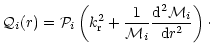
![\begin{figure}
\includegraphics[width=14cm]{2247f2.eps}
\end{figure}](/articles/aa/full/2001/27/aah2247/img98.gif) |
Figure 2:
Propagation diagram for Polytropic models of
index
|
The
standard second-order differential equation of linear adiabatic stellar oscillations
(Eq. (4)), can be written into a pair of self-adjoint differential
equations. As we will discuss later, these equations should then be regarded as being
complementary to each other, for the study of the local properties,
related with the two driving mechanisms, pressure and gravity.
The transformation of the second-order differential equation into a
self-adjoint form will be done, taking into account the previous decomposition
related with the two propagation cavities for a given wave.
This is accomplished by the transformation,
| (30) |
 |
(31) |
These complementary equations will be very useful in the
analysis of the zeros of
the wave function, ![]() .
The location of the turning points will determine
what is the most convenient formulation to study the properties
of a given wave of frequency,
.
The location of the turning points will determine
what is the most convenient formulation to study the properties
of a given wave of frequency,
![]() and degree, l, i.e., the formulation is chosen such that
and degree, l, i.e., the formulation is chosen such that
![]() is strictly positive
in the interval considered.
In fact, the localization of the singular points
depends on
is strictly positive
in the interval considered.
In fact, the localization of the singular points
depends on ![]() and l, and they correspond to the zeros of
and l, and they correspond to the zeros of
![]() or
or
![]() .
Choosing the convenient self-adjoint formulation for a given wave of
parameters
.
Choosing the convenient self-adjoint formulation for a given wave of
parameters ![]() and l, the function
and l, the function
![]() is regular (
is regular (
![]() )
in the interval
considered.
In this sense, in waves for which
)
in the interval
considered.
In this sense, in waves for which
![]() (
(
![]() )
in all
the interval (acoustic type), the location of zeros of
)
in all
the interval (acoustic type), the location of zeros of ![]() ,
corresponds to the location of zeros of
,
corresponds to the location of zeros of
![]() ,
provided that
,
provided that
![]() does not have zeros on the interval considered.
Equation (29)
with i=1, is the convenient formulation to study the oscillatory motions.
Conversely, in waves for which
does not have zeros on the interval considered.
Equation (29)
with i=1, is the convenient formulation to study the oscillatory motions.
Conversely, in waves for which
![]() (
(
![]() )
in
the interval considered (gravity type), the location of zeros of
)
in
the interval considered (gravity type), the location of zeros of ![]() corresponds to the location of zeros of
corresponds to the location of zeros of
![]() .
Equation (29)
with i=2, is then the convenient formulation to study the oscillatory motions.
As we will discuss in Sect. 3.2, for some l and
.
Equation (29)
with i=2, is then the convenient formulation to study the oscillatory motions.
As we will discuss in Sect. 3.2, for some l and ![]() a mixing mode can appear and both descriptions will need to be used.
Under a correct choice of the self-adjoint form, the differential
Eq. (4)
for each of the propagative regions,
the number and the location of the zeros of
a mixing mode can appear and both descriptions will need to be used.
Under a correct choice of the self-adjoint form, the differential
Eq. (4)
for each of the propagative regions,
the number and the location of the zeros of ![]() ,
can all be determined from a convenient self-adjoint form, even in such case.
,
can all be determined from a convenient self-adjoint form, even in such case.
In the following sections, when we are referring to a particular
formulation, we will use the underscript i on the
variables
![]() ,
,
![]() and
and
![]() ,
with i=1 for the
acoustic description and i=2 for the gravity description.
This is a first step to the classification scheme that
will be defined like it was originally proposed by Cowling (1941),
taking into account
the two driving mechanisms, the gravity and the pressure.
,
with i=1 for the
acoustic description and i=2 for the gravity description.
This is a first step to the classification scheme that
will be defined like it was originally proposed by Cowling (1941),
taking into account
the two driving mechanisms, the gravity and the pressure.
The phase analysis proposed here,
can be considered as a generalization of the method proposed by Eckart (1960),
Scuflaire (1974), Osaki (1975), Gabriel & Scuflaire (1979)
and Gough (1993) to discuss the classification scheme
of stellar oscillations.
The method proposed by these authors is
based on the algebraic counting of the number of nodes according to the
behaviour of p' relatively to ![]() (or the other two wave functions).
In our case the classification scheme will be determined for a generic wave function that
can be related with
(or the other two wave functions).
In our case the classification scheme will be determined for a generic wave function that
can be related with ![]() (for example), and the order of the mode will be determined
by the boundary conditions which can be, or not, reliable with the number of nodes
of this wave function.
(for example), and the order of the mode will be determined
by the boundary conditions which can be, or not, reliable with the number of nodes
of this wave function.
The motion equation for linear adiabatic nonradial oscillations (Eq. (4))
can be transformed into
two self-adjoint differential equations (Eq. (29))
to determine the properties of the oscillations.
Using the phase transformation (with i=1, 2) for each of the self-adjoint forms
(see details about this phase analysis in Appendix A),
given by
 |
(38) |
![$\displaystyle R_1
=R_{1,{\rm o}}\exp{\left[
\frac{1}{2}
\int_{r_{\rm o}}^r
\lef...
...}-{\cal T}(f_{\rm g})
\right)
\sin{\left(2\theta_1\right)} \; {\rm d}r
\right]}$](/articles/aa/full/2001/27/aah2247/img126.gif) |
(39) |
![$\displaystyle R_2
=R_{2,{\rm o}}\exp{\left[
\frac{1}{2}
\int_{r_{\rm o}}^r
\lef...
...}-{\cal T}(f_{\rm p})
\right)
\sin{\left(2\theta_2\right)} \; {\rm d}r
\right]}$](/articles/aa/full/2001/27/aah2247/img127.gif) |
(40) |
At this level, it is important to point out that Eqs. (36)
and (37) are two different phase representations of the same physical
system described by Eq. (4), written in a way that it avoids singular points
for a given wave of degree l and frequency ![]() ,
in a given region.
It is possible to determine a relation between
the two phases, which is obtained by imposing a matching of the logarithmic derivatives
of
,
in a given region.
It is possible to determine a relation between
the two phases, which is obtained by imposing a matching of the logarithmic derivatives
of ![]() (Eq. (28)) between both descriptions. This is given by
(Eq. (28)) between both descriptions. This is given by
 |
(41) |
In short, the propagation of a wave of degree l and frequency
![]() can be explicitly determined for any of the three types of waves
(which can be defined from the propagation diagrams)
using the appropriate phase equation.
For the pure acoustic type waves, the phase can be determined from
Eq. (36) (acoustic description) because no singular points occur
inside.
can be explicitly determined for any of the three types of waves
(which can be defined from the propagation diagrams)
using the appropriate phase equation.
For the pure acoustic type waves, the phase can be determined from
Eq. (36) (acoustic description) because no singular points occur
inside.
For the pure gravity type waves, the phase can be determined by Eq. (37) (gravity description). Furthermore, for mixed type waves which correspond to a mode that propagates in two different regions, Eq. (36) can be used to determine the phase propagation on the gravity region and Eq. (37) to determine the phase propagation on the acoustic region.
The matching condition is made in the region where both descriptions,
are accepted (without singular points). A possible choise is a point ![]() ,
where
,
where
![]() and
and
![]() ,
in that case from Eq. (42)
we obtain
,
in that case from Eq. (42)
we obtain
![]() .
To make the matching we integrate each of
the equations from each side of the interval and match them in the point
.
To make the matching we integrate each of
the equations from each side of the interval and match them in the point ![]() ,
where both solutions are valid.
,
where both solutions are valid.
The stellar oscillation eigenmodes can be determined by using one of the phase equations (Eqs. (36) or (37)), with a convenient set of boundary conditions at the endpoints, the centre and the surface. The phase equations are equivalent one another and the choice of which discription to use is matter of the tast of the author as well the type of singularities that can be enconter. Indeed, a certain phase equation with the respective boundary conditions at the center and the surface, constitutes an eigen-value problem. In the following, we will indicate how it is possible to determine the boundary conditions for each representation.
The phase at the endpoints is determined by using one of two procedures.
One consists in transforming the boundary conditions
of the eigenfunction ![]() or
or ![]() (see Sect. 2.2) into an equivalent endpoint condition
for the phase function
(see Sect. 2.2) into an equivalent endpoint condition
for the phase function ![]() of the phase associated system, related with
the differential Eq. (29).
Independent of the approximation made on the
determination of the local wavenumber, defined on
the equation of motion (see Sect. 2),
it is possible to determine the phase at the endpoints
from the Lagrangian perturbation of pressure
of the phase associated system, related with
the differential Eq. (29).
Independent of the approximation made on the
determination of the local wavenumber, defined on
the equation of motion (see Sect. 2),
it is possible to determine the phase at the endpoints
from the Lagrangian perturbation of pressure ![]() and the Eq. (A.5).
In the Appendix B, we present the determination of the boundary condition
in the case of the planar approximation (Deubner & Gough 1984).
and the Eq. (A.5).
In the Appendix B, we present the determination of the boundary condition
in the case of the planar approximation (Deubner & Gough 1984).
An alternatively method consists in determining the phase at the endpoints
by imposing the regularity of the phase function ![]() .
A detailed analysis of the phase Eqs. (36) and (37),
indicates that these ones are singular at the endpoints, r=0 (for all stars)
and r=R (only for polytropes).
This implies that the boundary conditions must be applied
such that the singular solution at each of the endpoints is eliminated.
This is obtained by expanding the solution,
.
A detailed analysis of the phase Eqs. (36) and (37),
indicates that these ones are singular at the endpoints, r=0 (for all stars)
and r=R (only for polytropes).
This implies that the boundary conditions must be applied
such that the singular solution at each of the endpoints is eliminated.
This is obtained by expanding the solution, ![]() ,
as a power series of r, relatively to the critical endpoint.
It is necessary also to expand the equilibrium quantities
around the endpoints, r=0 and r=R.
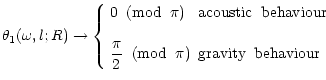
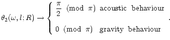
It is worth to notice that for each description it is possible to
study the properties of the gravity waves, as well as of the acoustic waves, even if
it is more convenient to use a gravity description to study the eigenstates
of gravity perturbations and similarly the acoustic description to study the eigenstates
of acoustic perturbations. In that case for each description, we will refered to the perturbation
as characterized by the main contributer for the restoring force
that is present in a certain region inside the star. In this context, we will refered
to an acoustic behaviour or the gravity behaviour,
as it is the gravity or the pressure the main contributer for the restoring force.
The mixed modes can be treated as a combination of these two "asymptotic'' cases
(as discussed in the previous section),
as an acoustic type mode or gravity type mode for each of the region where one
of these character prevails.
In particular, the inner and outer boundary conditions
for mixed modes are determined based in which is the dominant wave
character near the center or
near the surface of the star.
,
as a power series of r, relatively to the critical endpoint.
It is necessary also to expand the equilibrium quantities
around the endpoints, r=0 and r=R.
It is worth to notice that for each description it is possible to
study the properties of the gravity waves, as well as of the acoustic waves, even if
it is more convenient to use a gravity description to study the eigenstates
of gravity perturbations and similarly the acoustic description to study the eigenstates
of acoustic perturbations. In that case for each description, we will refered to the perturbation
as characterized by the main contributer for the restoring force
that is present in a certain region inside the star. In this context, we will refered
to an acoustic behaviour or the gravity behaviour,
as it is the gravity or the pressure the main contributer for the restoring force.
The mixed modes can be treated as a combination of these two "asymptotic'' cases
(as discussed in the previous section),
as an acoustic type mode or gravity type mode for each of the region where one
of these character prevails.
In particular, the inner and outer boundary conditions
for mixed modes are determined based in which is the dominant wave
character near the center or
near the surface of the star.
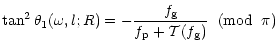
The inner boundary condition near the center is obtained by imposing that the solution to the phase
equation is regular, i.e. ![]() has a finite value. Now, we will illustrate that by considering
the case corresponding to the acoustic description, i.e., we are interested in determine the
solution,
has a finite value. Now, we will illustrate that by considering
the case corresponding to the acoustic description, i.e., we are interested in determine the
solution, ![]() as given by Eq. (36). Furthermore, we will starting by
considering a wave that has an acoustic behaviour near the stellar center,
it follows that
as given by Eq. (36). Furthermore, we will starting by
considering a wave that has an acoustic behaviour near the stellar center,
it follows that ![]() must be a regular function at the center, as the phase has a finite value.
We notice that the first-member of Eq. (36) is singular, consequently, the
finite value of
must be a regular function at the center, as the phase has a finite value.
We notice that the first-member of Eq. (36) is singular, consequently, the
finite value of
![]() is obtained by choosing all the multi-value solutions,
such as
is obtained by choosing all the multi-value solutions,
such as
![]() where n is a positive or a negative integer
(or in an equivalent form
where n is a positive or a negative integer
(or in an equivalent form
![]() ;
see also Appendix B). Similary in the
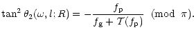
case of the gravity description (Eq. (36)),
a wave with a gravity behaviour at the center has a regular solution
if
;
see also Appendix B). Similary in the
case of the gravity description (Eq. (36)),
a wave with a gravity behaviour at the center has a regular solution
if
![]() .
It follows that the same boundary conditions
can be presented in both descriptions, given that
.
It follows that the same boundary conditions
can be presented in both descriptions, given that
![]() .
This relation between phases is illustrated in the next section.
In resume, the boundary condition for the center require
that
.
This relation between phases is illustrated in the next section.
In resume, the boundary condition for the center require
that
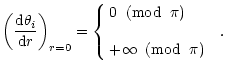 |
(43) |
The outer boundary condition, can be obtained also by a series expansion
around the endpoint r=R.
In the case of polytropic equilibrium structures,
because the sound speed is zero at r=R, the
phase Eqs. (36) and (37) can be singular. It follows that
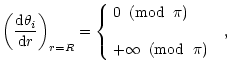 |
(46) |
 |
(49) |
 |
(50) |
We observe that with these boundary conditions for the inner endpoint, in both descriptions both solutions are regular because the amplitude and the phase have finite values for r=0.
Ledoux & Walraven (1958) have derived a particular solution,
which presents two asymptotic limits for very high
and very small eigenfrequencies. In this case the system of stellar oscillations under the
Cowling approximation tends toward a Sturm-Liouville type solution.
Here, an analogous situation takes place, when the term with the form
![]() ,
in Eqs. (36) and (37) can be neglected.
This is a good approximation in most of the stellar interior,
because this term remains small compared with
the other terms almost everywhere, except near the turning points
(where
,
in Eqs. (36) and (37) can be neglected.
This is a good approximation in most of the stellar interior,
because this term remains small compared with
the other terms almost everywhere, except near the turning points
(where ![]() or
or ![]() becomes 0)
and the stellar surface.
In that case,
the nodes of
becomes 0)
and the stellar surface.
In that case,
the nodes of
![]() (or
(or
![]() )
correspond
to extremes of
)
correspond
to extremes of
![]() (or
(or
![]() ).
The phase equations take the simple form:
).
The phase equations take the simple form:
It is important to stress that this is a very good representation for
the phase equations and from that we can say that the difference between the
acoustic and gravity waves presents a shift of ![]() .
In this case, it is very clear the fact that both phase equations are strictly
equivalent.
.
In this case, it is very clear the fact that both phase equations are strictly
equivalent.
For a given l, if ![]() is large this suggests the existence of
a spectrum of indefinitely increasing eigenvalues, corresponding to the eigensolution denoted by
acoustic modes or p-modes.
Conversely, for
is large this suggests the existence of
a spectrum of indefinitely increasing eigenvalues, corresponding to the eigensolution denoted by
acoustic modes or p-modes.
Conversely, for ![]() very small, this tends to define a Sturm-Liouville problem with
the parameter
very small, this tends to define a Sturm-Liouville problem with
the parameter
![]() ,
which
corresponds to the eigensolutions denoted by gravity modes or g-modes.
,
which
corresponds to the eigensolutions denoted by gravity modes or g-modes.
Copyright ESO 2001
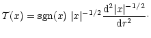
![$\displaystyle \frac{\rm d}{{\rm d}r}\left[{\cal P}_i (r) \frac{{\rm d}{\cal Y}_i}{{\rm d}r}\right] + {\cal Q}_i(r) {\cal
Y}_i=0,$](/articles/aa/full/2001/27/aah2247/img102.gif)