

Up: Nonradial adiabatic oscillations of
Subsections
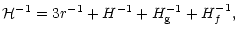
2 Basic equation of oscillatory motion
Formally, the nonradial adiabatic oscillations of stars can be described as
the solution of the simple linear homogeneous adiabatic wave equation:
![$\displaystyle {\put(0,0){\framebox (6,6){$\;\;$ }}}\hspace{0.3cm}\Psi=\left[\frac{\partial^2}{\partial t^2}+{\cal L} \right]\Psi =0$](/articles/aa/full/2001/27/aah2247/img18.gif) |
|
|
(1) |
where
 is the adiabatic wave operator and
 is some wave function depending on the position vector
  and
the time t, that characterizes the oscillations (Gough 1993, 1996).
The oscillatory motion under study is supposed to be of such low amplitude
that linearization of the full equations of fluid dynamics is valid,
allowing to determine the wave equation that describes the oscillatory
movements.
and
the time t, that characterizes the oscillations (Gough 1993, 1996).
The oscillatory motion under study is supposed to be of such low amplitude
that linearization of the full equations of fluid dynamics is valid,
allowing to determine the wave equation that describes the oscillatory
movements.
Therefore, we are ignoring the interactions between waves,
non-adiabatic effects which are important only in beneath the atmosphere,
and effects of the turbulence in the convective zone. We also consider
a non-magnetic and non-rotating star.
The adiabatic wave operator
depends on the structure of the solar model,
which we will refer to as the background state.
We have assumed that a frame of reference exists in which the background state
is independent of time.
In this case, there are genuinely separable solutions
![$\Psi(\vec{r},t)={\cal R}\left[ \Psi(\vec{r}) {\rm e}^{-i\omega t} \right]$](/articles/aa/full/2001/27/aah2247/img22.gif) of the simple homogeneous adiabatic equation.
Considering that the wave has a pure dependence on t with frequency
of the simple homogeneous adiabatic equation.
Considering that the wave has a pure dependence on t with frequency  ,
the spatial part of the wave function,
,
the spatial part of the wave function,
 satisfies:
 |
|
|
(2) |
where the three-dimensional spatial differential operator
 is obtained from the full wave operator
by replacing
is obtained from the full wave operator
by replacing
 by
by  .
We will use
.
We will use 
![[*]](/icons/foot_motif.gif) to represent the factor depending on r in the separated
form
to represent the factor depending on r in the separated
form
 with respect to the
spherical polar coordinates
with respect to the
spherical polar coordinates
 when the background state is spherically
symmetric, and where
when the background state is spherically
symmetric, and where
 is a spherical harmonic of degree l and azimuthal order m,
Pml being the associated Legendre function of first kind.
In this case, the separation of variables into radial
and angular parts is possible for all background variables,
with the angular dependence of
is a spherical harmonic of degree l and azimuthal order m,
Pml being the associated Legendre function of first kind.
In this case, the separation of variables into radial
and angular parts is possible for all background variables,
with the angular dependence of
 satisfying
the eigenvalue equation,
satisfying
the eigenvalue equation,
 |
|
|
(3) |
where
 is the horizontal Laplace operator,
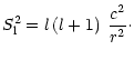
m=-l,...,+l and
L2=l(l+1).
In that case
will represent the radial part
of the corresponding three-dimensional operator with the same name.
In the spherically symmetric case, the solutions of Eq. (2)
together with appropriate boundary conditions, admit discrete eigenfrequencies
is the horizontal Laplace operator,
m=-l,...,+l and
L2=l(l+1).
In that case
will represent the radial part
of the corresponding three-dimensional operator with the same name.
In the spherically symmetric case, the solutions of Eq. (2)
together with appropriate boundary conditions, admit discrete eigenfrequencies
 ,
where n is the radial wave number.
The spherical symmetry of the background state is responsable
by the degeneracy of
with respect to m.
,
where n is the radial wave number.
The spherical symmetry of the background state is responsable
by the degeneracy of
with respect to m.
In the case of a spherically symmetrical background state, the homogeneous differential
equation (Eq. (2)) representing adiabatic oscillations is of fourth-order and has
to be solved subject to two regularity conditions at the coordinate singularity
r=0, and to two boundary conditions at the surface r=R (Unno et al. 1989; Gough 1993).
Taking into account the mathematical structure of the operator
,
it is possible to reduce this one to the
standard second-order differential equation.
This equation of motion can be obtained directly from
a linearized Eulerian momentum equation and from the Poisson equation
that describes the oscillatory motion
by making a convenient transformation (Gough 1993).
In the following, we make a very brief presentation of
approximations to the second-order motion equations.
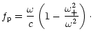
2.1 The standard form
The linear adiabatic nonradial stellar oscillations
of a spherically symmetrical background state can be written in
a standard form. Generically we can write the motion equation
of adiabatic nonradial oscillations as
 |
|
|
(4) |
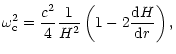
where the radial component of the local wave number,  ,
is given by
,
is given by
 |
|
|
(5) |
where c, is the radial distribution of sound speed,
 ,
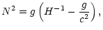
defines a generalized critical frequency and
,
defines a generalized critical frequency and  ,
a generalized Brunt-Väisälä frequency,
that takes into account the geometrical terms and gravity
contribution for the local wave number,
which will be defined for each of the approximative motion equations.
is the
wave function, which is proportional to the Lagrangian perturbation
of pressure and will take a particular dependence, in agreement with
the approximation used.
,
a generalized Brunt-Väisälä frequency,
that takes into account the geometrical terms and gravity
contribution for the local wave number,
which will be defined for each of the approximative motion equations.
is the
wave function, which is proportional to the Lagrangian perturbation
of pressure and will take a particular dependence, in agreement with
the approximation used.
In the following analysis we will always consider this general case
given by Eq. (4),
unless we say explicitly the contrary.
2.1.1 The Planar approximation
In 1984, Deubner & Gough determined a linear second-order differential
equation in the standard form of the Eq. (4),
to describe the dynamics of adiabatic non-radial oscillations.
This equation of motion has been obtained by a procedure
analogous to the Lamb (1932) method. This approximation can be
made for waves with wavelength much smaller than the solar radius
and where the local effects of spherical geometry on the oscillatory
motion can be ignored. Additionally, the perturbations of the gravitational
potential have been ignored.
In this case, the wave function is given by,
 |
|
|
(6) |
where  ,
is the density and
,
is the density and  ,
is the Lagrangian
perturbation of pressure. In this case,
the local wave number, ,
is given by Eq. (5),
where the critical frequency,
,
is given by
,
is the Lagrangian
perturbation of pressure. In this case,
the local wave number, ,
is given by Eq. (5),
where the critical frequency,
,
is given by
 |
|
|
(7) |
where H, is the density scale height.
The generalized Brunt-Väisälä frequency, ,
is reduced to the classical Brunt-Väisälä frequency, N,
given by
 |
|
|
(8) |
where g, is the gravitational acceleration.
This model is particularly interesting because of the simplicity in the
interpretation of the characteristic frequencies of the equilibrium structure
that determine the cavities of propagative waves.
All the main properties of the local behavior of waves,
can be well defined in this approximation.
The equation of motion of stellar oscillations can be obtained by
reducing the fourth-order system of stellar oscillations to a second-order
differential equation, where the Eulerian perturbation of
the gravitational potential is neglected (Gough 1993). Cowling (1941)
showed the interest of this approximation, by
pointing out that it has a relatively minor effect on the modes,
with exception to the modes of low degree and low order.
Under the approximation proposed, i.e., neglecting
the contribution of the Eulerian pertubation of gravitational potential,
 ,
the initial fourth-order system of adiabatic stellar oscillations
is reduced to a second-order motion equation,
by the following transformation
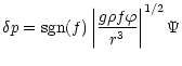
,
the initial fourth-order system of adiabatic stellar oscillations
is reduced to a second-order motion equation,
by the following transformation
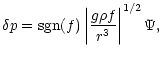 |
|
|
(9) |
where sgn(f), is the sign of the discriminant f.
This discriminant, is given
by
 |
|
|
(10) |
 ,
is the square of the Jeans frequency,
that is equal to
,
is the square of the Jeans frequency,
that is equal to
 ,
where G is the gravitational
constant.
Using this transformation, the motion equation of
adiabatic nonradial stellar oscillations,
can be written in the form of Eq. (4).
In that case, the generalized Brunt-Väisälä frequency,
,
is given by
,
where G is the gravitational
constant.
Using this transformation, the motion equation of
adiabatic nonradial stellar oscillations,
can be written in the form of Eq. (4).
In that case, the generalized Brunt-Väisälä frequency,
,
is given by
 |
|
|
(11) |
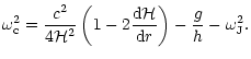
and the critical frequency,
,
is given by
 |
|
|
(12) |
where
h is the scale height of g/r2 and
 is a generalized scale height.
The scale height h, is given by
is a generalized scale height.
The scale height h, is given by
 |
|
|
(13) |
and
,
is given by
 |
|
|
(14) |
where  ,
is the gravity scale height and Hf, is the
scale height of discriminant f.
A detailed discussion about these variables is presented in Gough (1993).
,
is the gravity scale height and Hf, is the
scale height of discriminant f.
A detailed discussion about these variables is presented in Gough (1993).
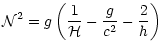
The difference between the generalization of the Brunt-Väisälä frequency,
and
the critical frequency,
relatively to these quantities
in the Deubner & Gough (1984) approach,
is due to the contribution of geometrical terms,
that can be important for the most penetrative modes in very
dense stars.
A more general solution to the initial system of stellar
oscillations can be obtained, which takes into
account a major contribution related with  .
This is called the first Post-Cowling approximation
(Gough 1993; Dziembowski & Gough, private comunication). Under this approximation the
Brunt-Väisälä frequency, ,
is given by
.
This is called the first Post-Cowling approximation
(Gough 1993; Dziembowski & Gough, private comunication). Under this approximation the
Brunt-Väisälä frequency, ,
is given by
 |
|
|
(15) |
and the critical frequency,
,
is given by
The total scale height ,
is given by
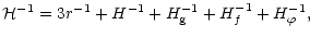 |
|
|
(16) |
where the scale height
 takes into account
the contribution related with the
perturbation of the gravitational potential (Gough 1993;
Dziembowski & Gough, private comunication; Lopes 2001). The scale height
,
is given by
takes into account
the contribution related with the
perturbation of the gravitational potential (Gough 1993;
Dziembowski & Gough, private comunication; Lopes 2001). The scale height
,
is given by
 |
|
|
(17) |
The wave function, ,
can be determined as
 |
|
|
(18) |
where  ,
is a structure term related with the background state,
given by
,
is a structure term related with the background state,
given by
 |
|
|
(19) |
These new expressions
for the characteristic frequencies come from a contribution related with the perturbation of
the gravitational potential which can be obtained from the linearized
Poisson equation. The magnitude of the effect relatively to the
classical Cowling approximation strongly depends on the density distribution
in the central region of the star.
2.2 Boundary conditions
The second-order motion equation together with two boundary
conditions, one at the centre and the other at the surface, forms
an eigen-value problem. We will present these boundary conditions
here, as they will be needed later.
The center is a regular singular point.
The regularity condition for the perturbation of
the Lagrangian variation of pressure, ,
is given by
 |
|
|
(20) |
as
 .
The outer boundary condition, is fixed in the atmosphere
and we consider that the inertia of the corona is so high
that ,
is given approximately by
.
The outer boundary condition, is fixed in the atmosphere
and we consider that the inertia of the corona is so high
that ,
is given approximately by
 |
|
|
(21) |
at r=R.
These simple conditions are sufficient to the discussion proposed
in this article.
These are the so-called "zero-boundary conditions'' (Unno et al. 1989).
The consideration of more realistic boundary
conditions does not modify significantly the method proposed to classify
modes in stars.
2.3 Propagation diagram
![\begin{figure}
\includegraphics[width=14cm]{2247f1.eps}
\end{figure}](/articles/aa/full/2001/27/aah2247/Timg69.gif) |
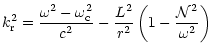
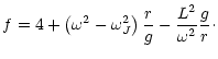
Figure 1:
Propagation diagram for a polytropic model with
index
 ,
adiabatic index ,
adiabatic index
 .
The curves correspond to a dimensionless circular frequency
relatively to the dimensionless radius.
These curves delimit the propagation region for modes of
degree .
The curves correspond to a dimensionless circular frequency
relatively to the dimensionless radius.
These curves delimit the propagation region for modes of
degree  :
a) The solid curves represent :
a) The solid curves represent
 computed in the Cowling approximation,
the dashed curves represent planar values of
,
and the dotted curves represent the Brünt-Väisäla frequency, N,
(increasing from the center to the surface) and the Lamb frequency,
computed in the Cowling approximation,
the dashed curves represent planar values of
,
and the dotted curves represent the Brünt-Väisäla frequency, N,
(increasing from the center to the surface) and the Lamb frequency,  ,
(decreasing from the center to the surface).
b) The solid curves represent
computed in
the first Post-Cowling approximation, and the dashed curve represents
in the Cowling approximation. ,
(decreasing from the center to the surface).
b) The solid curves represent
computed in
the first Post-Cowling approximation, and the dashed curve represents
in the Cowling approximation. |
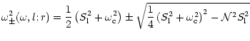
The direction and magnitude of the acoustic-gravity wave is determined by the
competition between the radial and tangential components of
the local wave number  ,
given by
,
given by
 |
|
|
(22) |
where
 ,
,
 are unitary vectors in the
radial and horizontal directions and
are unitary vectors in the
radial and horizontal directions and
 (
(
 ), is the tangential component of the local wave number (Unno et al. 1989). The radial component of the local wave number,
is determined by the local properties of the equilibrium structure.
In this sense, it is possible to build a diagram for the radial component of the local
wave number, which defines the regions of propagative or evanescent behavior
of a given acoustic-gravity wave of frequency
and degree l.
This is the so-called propagation diagram.
Waves can propagate where the square of the vertical component of the local wave
is greater than zero, and are evanescent elsewhere.
This leads to two asymptotic limits, for the very high and for the very small
frequencies. In the case of very high frequencies,
), is the tangential component of the local wave number (Unno et al. 1989). The radial component of the local wave number,
is determined by the local properties of the equilibrium structure.
In this sense, it is possible to build a diagram for the radial component of the local
wave number, which defines the regions of propagative or evanescent behavior
of a given acoustic-gravity wave of frequency
and degree l.
This is the so-called propagation diagram.
Waves can propagate where the square of the vertical component of the local wave
is greater than zero, and are evanescent elsewhere.
This leads to two asymptotic limits, for the very high and for the very small
frequencies. In the case of very high frequencies,
 ,
the propagation
is predominantly in the radial direction. In the other case,
,
the propagation
is predominantly in the radial direction. In the other case,
 ,
then the propagation is predominantly in the horizontal direction.
This corresponds also to the spectral regions
where the restoring forces are dominated by gravity
(through the buoyancy) or pressure.
Because of that, it is convenient to write the local
wave number as a function of the critical frequencies
,
in which case ,
is given by
,
then the propagation is predominantly in the horizontal direction.
This corresponds also to the spectral regions
where the restoring forces are dominated by gravity
(through the buoyancy) or pressure.
Because of that, it is convenient to write the local
wave number as a function of the critical frequencies
,
in which case ,
is given by
 |
|
|
(23) |
where  is a discriminant, given by
 |
|
|
(24) |
and  is a discriminant, given by
 |
|
|
(25) |
The underscript g or p is fixed by the propagative regions that
are separated by
 or
or
 ,
respectively.
,
respectively.
It follows from Eq. (23) that
 ,
are real and
,
are real and
 and
and
 (acoustic or p-region, locally behaves like an acoustic type wave) or
 and
and
 (gravity or g-region, locally behaves like a gravity type wave). Here we will be mainly concerned with the case where
 and
and
 are both real.
In the case where
and
are complex conjugates
it is also possible to use the same analysis.
It will slightly complicate the algebra, but the physical conclusions remain the same.
are both real.
In the case where
and
are complex conjugates
it is also possible to use the same analysis.
It will slightly complicate the algebra, but the physical conclusions remain the same.
The critical frequencies
,
define the turning points of the
standard second-order differential equation,
previously presented, i.e.,
 .
In the more general case,
,
can be determined numerically. However
the critical frequencies
.
In the more general case,
,
can be determined numerically. However
the critical frequencies
 can be obtained,
by the relation,
can be obtained,
by the relation,
 |
|
|
(26) |
where, the Lamb frequency  ,
is given by
,
is given by
 |
|
|
(27) |
In the case of Deubner & Gough (1984),
these expressions determine an explicit relation
of the critical frequencies as function
of the background structure and independent of the frequency
(see Sect. 2.1.1).
In Figs. 1 and 2 we present
the
computed critical frequencies,
,
for
the different approximations presented in the previous section,
in the case of polytropes of index
 and
and
 and adiabatic
index
.
A discussion about the
propagation of waves in polytropic equilibrium structure
with a different adiabatic index can be found in
Cowling (1941) and Scuflaire (1974).
The contribution related with the geometric
terms occuring in the variables
and
when
computed in the Cowling approximation is more important
for the more penetrative waves, i.e., waves with smaller degree,
as it is illustrated in Figs. 1a and 2a.
Similarly, the first Post-Cowling approximation,
seems worth considering in the case of stars with high density,
where the presence of the gravitational potential modifies
significantly the values of
in the central
region of the star
(cf. Figs. 1b and 2b).
and adiabatic
index
.
A discussion about the
propagation of waves in polytropic equilibrium structure
with a different adiabatic index can be found in
Cowling (1941) and Scuflaire (1974).
The contribution related with the geometric
terms occuring in the variables
and
when
computed in the Cowling approximation is more important
for the more penetrative waves, i.e., waves with smaller degree,
as it is illustrated in Figs. 1a and 2a.
Similarly, the first Post-Cowling approximation,
seems worth considering in the case of stars with high density,
where the presence of the gravitational potential modifies
significantly the values of
in the central
region of the star
(cf. Figs. 1b and 2b).
In the next section, using the differential Eq. (4) with the local
wave number given by Eq. (23), we will
write the standard equation of motion
in a convenient self-adjoint form, very appropriate for
the phase analysis that we will present below.
Up: Nonradial adiabatic oscillations of
Copyright ESO 2001
![\begin{figure}
\includegraphics[width=14cm]{2247f1.eps}
\end{figure}](/articles/aa/full/2001/27/aah2247/img69.gif)