For the sake of analysis and discussion, we transform the dust moment
equations derived in Sects. 5.1 and 5.2
into their dimensionless form by introducing reference values as
 ,
,
 ,
,
 ,
,
 ,
,
 ,
,
 ,
,
 ,
,
 ,
,
 ,
,
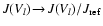
 following the procedure described in Paper I. The reference values are to be
chosen according to the expected order of magnitude of the respective
quantities and the length and time-scales under investigation. After this
substitution, all quantities are dimensionless and can be compared by number.
following the procedure described in Paper I. The reference values are to be
chosen according to the expected order of magnitude of the respective
quantities and the length and time-scales under investigation. After this
substitution, all quantities are dimensionless and can be compared by number.
This allows us to identify the leading terms in the equations, e.g.in the inner and outer regions of a brown dwarf atmosphere. The remaining constants (products of the reference values) can be summarised into characteristic numbers which provide an efficient way to describe the qualitative behaviour of the dust component.
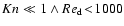
The dimensionless dust moment equations for nucleation, growth,
evaporation, and equilibrium drift write for a subsonic free
molecular flow (
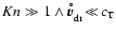 )
)
 )
)
 . The constants
in squared brackets are written in terms of characteristic numbers,
which are further explained in Table 2. All other
quantities and terms in Eqs. (77) and (78)
are of the order of unity for an appropriate choice of the reference
values.
. The constants
in squared brackets are written in terms of characteristic numbers,
which are further explained in Table 2. All other
quantities and terms in Eqs. (77) and (78)
are of the order of unity for an appropriate choice of the reference
values.
The following discussion is based on a typical structure of a brown
dwarf atmosphere with solar abundances in the gas phase, i.e.
neglecting the possible depletion due to dust formation (see
Table 2). As underlying ( )-structure we refer to a
brown dwarf model atmosphere with
)-structure we refer to a
brown dwarf model atmosphere with
 K and
K and
 which has been kindly provided by
T. Tsuji (2002)
which has been kindly provided by
T. Tsuji (2002)![[*]](/icons/foot_motif.gif) . As exemplary dust species we consider solid SiO2(amorphous quartz), growing by the accretion of SiO and H2O
(Eq. (38)). Since the nucleation of SiO2 seems
dubious (the monomer is rather unstable as a free molecule and hence
not very abundant in the gas phase) we consider nucleation of TiO2instead.
. As exemplary dust species we consider solid SiO2(amorphous quartz), growing by the accretion of SiO and H2O
(Eq. (38)). Since the nucleation of SiO2 seems
dubious (the monomer is rather unstable as a free molecule and hence
not very abundant in the gas phase) we consider nucleation of TiO2instead.
| Name | Characteristic | Value | ||||||
| Number | inside | outside | ||||||
| Mach number |
 |
 |
||||||
| Froude number |
 |
0.842 |
 |
0.495 |
 |
|||
| Strouhal number |
 |
 |
||||||
| hydrodyn. Knudsen number |
 |
 |
 |
 |
 |
|||
| Knudsen number (Eq. (6)) |
 |
 |
... |
 |
||||
| Drift number |
 |
 |
... |
 |
||||
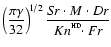
combined drift number (
 ) ) |
 |
 |
... |
 |
||||
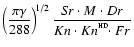
combined drift number (
 ) ) |
 |
 |
... |
 |
||||
 : 1 : 1 |
: 1 |
|||||||
Sedlmaÿr number
 |
 |
 : :
 |
:
 |
|||||
 : :
 |
:
 |
|||||||
 : :
 |
:
 |
|||||||
| Damköhler no. of nucleation |
 |
0 | 0 |
 |
 |
|||
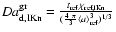
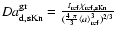
| Damköhler no. of growth (
) |
 |
3.95 |
 |
 |
 |
|||
| Damköhler no. of growth (
) |
 |
 |
 |
 |
 |
|||
| Name | Physical Quantity | Reference Value | ||||||
| inside | outside | |||||||
| temperature |
 |
[K] | 1700 | ... | 1000 | |||
| density |
 |
[g/cm3] |
 |
... |
 |
|||
| thermal pressure |
 |
[dyn/cm2] |
 |
... |
 |
|||
| velocity of sound |
 |
[cm/s] |
 |
... |
 |
|||
| velocity |
 |
[cm/s] |
 |
|||||
| length |
 |
[cm] | 10+4 | 10+6 | 10+4 | 10+6 | ||
| hydrodyn. time |
 |
[s] |
 |
 |
 |
 |
||
| gravitational acceleration |
 |
[cm/s2] | 10+5 | |||||
| mean particle radius |
 |
[cm] | 10-3 | ... | 10-6 |
 |
||
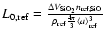
0th dust moment (
 ) ) |
 |
[1/g] |
 |
... |
 |
 |
||
| nucleation rate |
 |
[1/s] |
 |
... |
 |
|||
| growth velocity (
,
Eq. (67)) |
 |
[cm/s] |
 |
... |
 |
 |
||
| growth velocity (
,
Eq. (76)) |
 |
[cm2/s] |
 |
... |
 |
|
||
| diffusion constant (Eq. (26)) |
 |
[cm2/s] |
 |
... | 2.43 |
|
||
| mean free path (Eq. (10)) |
 |
[cm] |
 |
... |
 |
|||
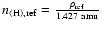
| total hydrogen number density |
 |
[1/cm3] |
 |
... |
 |
|||
| molecular number density |
 |
[1/cm3] |
 |
... |
 |
|
||
: According to the experience of Paper I.
: We choose the reference value of the dust-to-gas mass ratio
 by considering the case when all Si is
bound in solid SiO2 and adapt the referece value for the total dust
particle density
by considering the case when all Si is
bound in solid SiO2 and adapt the referece value for the total dust
particle density
 according to the assumed
grain's reference size
according to the assumed
grain's reference size
 :
:
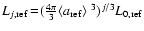 (Gail
(Gail
 Sedlmayr 1999).
 : We assume vanishing nucleation rates in this region
around 1700 K, because the supersaturation ratios
: We assume vanishing nucleation rates in this region
around 1700 K, because the supersaturation ratios  are either
too small for efficient nucleation or the nucleation species have already
been consumed by growth.
are either
too small for efficient nucleation or the nucleation species have already
been consumed by growth.
 : The reference value for the nucleation rate
 is chosen by considering homogeneous nucleation of TiO2 according to
Paper I.
: SiO is considered as key growth species.
is chosen by considering homogeneous nucleation of TiO2 according to
Paper I.
: SiO is considered as key growth species.
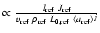
An analysis of the characteristic numbers in front of the source terms
in Eqs. (77) and (78) (see
Table 2) reveals a hierarchy of nucleation
 growth
drift:
growth
drift:
 )
and nucleation is effective
(
)
and nucleation is effective
(
 ). The products of the Damköhler number of
nucleation
). The products of the Damköhler number of
nucleation
 with the Strouhal number
  and the Sedlmaÿr
numbers
and the Sedlmaÿr
numbers  are as large as the products of the Damköhler numbers of growth
 with the Strouhal number
(even larger for small j) and
much larger than the combined drift numbers, indicating that the nucleation
provides an important source term in Eqs. (77) and
(78). Consequently, the condensable elements will be quickly
consumed by the process of nucleation before the particles can grow much
further. Hence, the dust particles remain very small in this layer of
effective nucleation.
)
and nucleation is not effective
(
with the Strouhal number
(even larger for small j) and
much larger than the combined drift numbers, indicating that the nucleation
provides an important source term in Eqs. (77) and
(78). Consequently, the condensable elements will be quickly
consumed by the process of nucleation before the particles can grow much
further. Hence, the dust particles remain very small in this layer of
effective nucleation.
)
and nucleation is not effective
(
 ). The products of the Damköhler numbers of growth
 with the Strouhal number
are large and the growth
term (the second term on the r.h.s.) is the leading source term in
the dust moment Eqs. (77) and (78).
In comparison, the influence of the drift term is small as
quantified by the combined drift numbers in
Table 2. Consequently, the dust growth process
will substantially be completed before the dust grains start to
settle gravitationally. In these growth-dominated layers,
a few existing particles will quickly consume all condensable
elements from the gas phase and, thus, will reach much larger
particle sizes. Since these particles cannot be created via
nucleation here, they must have been formed elsewhere and
transported into these layers by winds or drift. The growth will
either be terminated by element consumption or by the loss due to
gravitational settling when the particles reach their maximum size
as introduced in Sect. 3.1.
with the Strouhal number
are large and the growth
term (the second term on the r.h.s.) is the leading source term in
the dust moment Eqs. (77) and (78).
In comparison, the influence of the drift term is small as
quantified by the combined drift numbers in
Table 2. Consequently, the dust growth process
will substantially be completed before the dust grains start to
settle gravitationally. In these growth-dominated layers,
a few existing particles will quickly consume all condensable
elements from the gas phase and, thus, will reach much larger
particle sizes. Since these particles cannot be created via
nucleation here, they must have been formed elsewhere and
transported into these layers by winds or drift. The growth will
either be terminated by element consumption or by the loss due to
gravitational settling when the particles reach their maximum size
as introduced in Sect. 3.1.
 ). Consequently, nucleation and growth vanish
and the only remaining source term on the r.h.s. of
Eqs. (77) and (78) is the additional
advection of the particles due to their drift motion (drift term).
The combined drift numbers, however, are small indicating that the
drift term has a smaller influence than the hydrodynamical advection term.
). Consequently, nucleation and growth vanish
and the only remaining source term on the r.h.s. of
Eqs. (77) and (78) is the additional
advection of the particles due to their drift motion (drift term).
The combined drift numbers, however, are small indicating that the
drift term has a smaller influence than the hydrodynamical advection term.
| Name | Value | ||
| dust material density |
 |
[g/cm3] | 2.65 |
| monomer volume |
 |
[cm3] |
 |
| lower dust grain radius |
 |
[cm] |
 |
| molecular radius |
 |
[cm] |
 |
| physical process |
|
|
| time-derivative |
 |
|
| advective term | 1 | |
nucleation term
 |
 |
|
| growth term
|
 |
 |
| drift term |
 |
 |
|
: the importance of this process depends
on the considered dust moment j with the following associated mean dust quantity:  dust particle density,
 dust size,
 dust surface area,
 dust mass density.
|
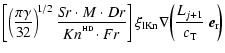
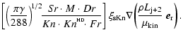
Table 4 shows some dependencies of the combined characteristic numbers (the squared brackets in Eqs. (77), (78)), which provides scaling laws for the importance of the different processes in the different regimes:
 (
)
or
(
)
or
 (
)
whereas the growth term scales as
(
)
whereas the growth term scales as
 with different
 for the different cases (Table 4). This
means that at a certain large mean particle size, the drift term
will start to dominate over growth, which in fact just occurs at
the maximum particle size
for the different cases (Table 4). This
means that at a certain large mean particle size, the drift term
will start to dominate over growth, which in fact just occurs at
the maximum particle size
 introduced in
Sect. 3.1.
)
become increasingly important with increasing gas density
(note that typically
introduced in
Sect. 3.1.
)
become increasingly important with increasing gas density
(note that typically
 with
with  ), whereas the drift term (
)
diminishes for increasing
,
i.e.the drift is
generally more important in a thin gas. However, the particles are
expected to remain smaller in such a thin gas situated in the upper
layers, which has a stronger, opposite effect on the
drift term.
,
the more stiff the dust moment equations become because of
the increasingly large nucleation and growth terms. This may
actually cause some numerical difficulties for models on macroscopic
scales. In comparison, the advective and the drift term are
independent on
,
which means that these terms gain
importance on small scales in relation to the other terms.
), whereas the drift term (
)
diminishes for increasing
,
i.e.the drift is
generally more important in a thin gas. However, the particles are
expected to remain smaller in such a thin gas situated in the upper
layers, which has a stronger, opposite effect on the
drift term.
,
the more stiff the dust moment equations become because of
the increasingly large nucleation and growth terms. This may
actually cause some numerical difficulties for models on macroscopic
scales. In comparison, the advective and the drift term are
independent on
,
which means that these terms gain
importance on small scales in relation to the other terms.
 ,
i.e.the drift is naturally
more important for heavy grains in a strong gravitational field.
,
i.e.the drift is naturally
more important for heavy grains in a strong gravitational field.
In Table 2, we have assumed
 ,
i.e.we have
considered time-scales
,
i.e.we have
considered time-scales
 of the order of
 ,
appropriate for disordered (e.g.turbulent)
velocity fields, where the l.h.s. terms of Eqs. (77) and
(78) are of comparable importance. However, if
large-scale systematic motions are stable for a long time (e.g.a
circulating thunderstorm or a stable convection roll), the system may
reach a quasi-stationary situation where
becomes much
larger and hence
,
appropriate for disordered (e.g.turbulent)
velocity fields, where the l.h.s. terms of Eqs. (77) and
(78) are of comparable importance. However, if
large-scale systematic motions are stable for a long time (e.g.a
circulating thunderstorm or a stable convection roll), the system may
reach a quasi-stationary situation where
becomes much
larger and hence
 .
In this case, the first
term on the l.h.s. of Eqs. (77) and (78)
vanishes (see Table 4) whereas all other terms remain
unaffected.
.
In this case, the first
term on the l.h.s. of Eqs. (77) and (78)
vanishes (see Table 4) whereas all other terms remain
unaffected.
An interesting special case occurs if additionally
 ,
i.e.when the dust-forming system reaches the static
case. In this case, also the advective terms in
Eqs. (77) and (78) vanish and the source
terms must balance each other. In the
,
i.e.when the dust-forming system reaches the static
case. In this case, also the advective terms in
Eqs. (77) and (78) vanish and the source
terms must balance each other. In the  case, this means that
the gain of dust by nucleation and growth must be balanced by the loss
of dust due to rain-out, which means that the gas will be depleted. In
the
case, this means that
the gain of dust by nucleation and growth must be balanced by the loss
of dust due to rain-out, which means that the gas will be depleted. In
the  case, just the opposite is true, i.e.the loss by
evaporation must be balanced by the gain of dust particles raining in
from above. Consequently, the gas in such undersaturated layers will
be enriched by the condensable elements liberated by the evaporating
grains.
case, just the opposite is true, i.e.the loss by
evaporation must be balanced by the gain of dust particles raining in
from above. Consequently, the gas in such undersaturated layers will
be enriched by the condensable elements liberated by the evaporating
grains.
However, both control mechanisms (in the static limit) result in an
efficient transport of condensable elements from the cool upper layers
into the warm inner layers, which cannot last forever. We may conclude
that if the brown dwarf's atmosphere is truly static for a long time,
there is no other than the trivial solution for
Eqs. (77) and (78) where the gas is
saturated (
 )
and dust-free (
)
and dust-free (
 ). This situation
changes, however, if the brown dwarf's atmosphere is turbulent or, in
particular, when it is convective. In that case, the replenishment of
the atmosphere with fresh uncondensed gas from the deep interior will
counteract the downward transport of condensable elements by the
formation and gravitationally settling of dust grains. Simulations of
this quasi-static balance will be the subject of the forthcoming paper
in this series.
). This situation
changes, however, if the brown dwarf's atmosphere is turbulent or, in
particular, when it is convective. In that case, the replenishment of
the atmosphere with fresh uncondensed gas from the deep interior will
counteract the downward transport of condensable elements by the
formation and gravitationally settling of dust grains. Simulations of
this quasi-static balance will be the subject of the forthcoming paper
in this series.
A dynamical modelling of the dust component in brown dwarf atmospheres
by means of a moment method as proposed in this paper - consistently
coupled to hydrodynamics, radiative transfer and element depletion in
the scope of hydrodynamical or classical stellar atmosphere
calculations - seems straightforward as soon as two major problems can
be solved:
or
,
where all grains fall into one particular case. This situation may be
relevant for the cool upper regions of a brown dwarf atmosphere, where
the densities are small and the dust particles remain tiny. In
general, however, a solution of this problem by means of a moment
method can only be approximate in nature and will require additional
numerical tricks, e.g.switching the case as soon as the Knudsen number
according to the mean size of the particles reaches unity.
)
or even Lj+2 (for
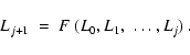
). Therefore, in order to benefit from the moment Eqs. (77) / (78), we require a physically
reliable closure condition, as e.g.
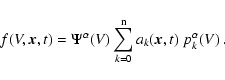
One idea to construct such a closure condition has been developed by
Deufelhard
Wulkow (1989) and Wulkow (1992),
studying the kinetics of polyreaction systems. The size distribution
function f(V) is here approximated by a weight function
 ,
which describes the basic shape of f(V), and
modified by a sum of orthogonal polynomials
,
which describes the basic shape of f(V), and
modified by a sum of orthogonal polynomials
 (k=0,1,2, ... ,n) as
 is an additional parameter (dependent on
  )
of the
weight function and ak are polynomial coefficients. The parameters
and ak
)
of the
weight function and ak are polynomial coefficients. The parameters
and ak
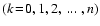 are stepwise adjusted in
order to fit the known moments Lj
are stepwise adjusted in
order to fit the known moments Lj
 exactly, using the orthogonality relation
 .
Once
these coefficients are known, all missing moments of the size
distribution function can be reconstructed from
Eq. (80), again utilising the orthogonality relation.
This procedure leads to reliable results, if the weight function
is already close to the actual size distribution
function f(V), such that the polynomials only provide small
corrections and the sum in Eq. (80) converges
rapidly.
.
Once
these coefficients are known, all missing moments of the size
distribution function can be reconstructed from
Eq. (80), again utilising the orthogonality relation.
This procedure leads to reliable results, if the weight function
is already close to the actual size distribution
function f(V), such that the polynomials only provide small
corrections and the sum in Eq. (80) converges
rapidly.
Copyright ESO 2003
![$\displaystyle \big[{S\!r}\big]\frac{{\rm\partial} }{{\rm\partial} t}\big(\rho L_j\big)$](/articles/aa/full/2003/07/aah3912/img407.gif)
![$\displaystyle \nabla ({\vec v}_{\rm gas}~\rho L_j)\;=\;
\big[{S\!r}\cdot{Da^{\rm nuc}_{\rm d}\!\cdot S\!e_{\rm j}}\big]~J({V_{\ell}})$](/articles/aa/full/2003/07/aah3912/img408.gif)
![$\displaystyle \left[{S\!r}\cdot{Da^{\rm gr}_{{\rm d}, lKn}}\right]\frac{j}{3}~
\chi^{\rm net}_{\rm lKn}~\rho L_{j-1}$](/articles/aa/full/2003/07/aah3912/img409.gif)
![$\displaystyle \left[{S\!r}\cdot{Da^{\rm gr}_{\rm d, sKn}}\right]\frac{j}{3}~
\chi^{\rm net}_{\rm sKn}~\rho L_{j-2}
\hfill$](/articles/aa/full/2003/07/aah3912/img412.gif)
 K and
K and
 K)
and an outer (
K)
and an outer (
 K) layer, typical for the
growth-dominated region and the region of effective nucleation,
respectively (see text). We assume constant
K) layer, typical for the
growth-dominated region and the region of effective nucleation,
respectively (see text). We assume constant
 and
and
 amu (
amu (
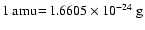 ).
In each layer, two reference length scales are considered:
).
In each layer, two reference length scales are considered:
 cm (microscopic scale) and
 cm (
cm (
 ;
macroscopic
scale). The reference values for the dust complex have been adopted
according to the experience of Paper I, considering an undepleted
gas of solar abundances. The growth rates are calculated for
SiO2 via addition of SiO and H2O (see
Eq. (
;
macroscopic
scale). The reference values for the dust complex have been adopted
according to the experience of Paper I, considering an undepleted
gas of solar abundances. The growth rates are calculated for
SiO2 via addition of SiO and H2O (see
Eq. ( and
and
 .
Further molecular and dust material quantities
are listed in Table
.
Further molecular and dust material quantities
are listed in Table