4 Thermal structure results

In this section we present the calculated thermal and ionization structure along wind flow lines, discuss the physical origin of the temperature plateau and its connection with the underlying MHD solution, discuss the effect of various key model parameters and finally compare our results with those found by Safier. The parameters spanned for the calculation of the thermal solutions are the wind ejection index $\xi$ describing the flow line geometry, the mass accretion rate $\dot{M}_{\rm acc}$ and the cylindrical radius $\varpi _0$ where the field is anchored in the disk.

4.1 Temperature evolution

In Fig. 2, solid curves present the out of ionization equilibrium evolution of temperature, electronic density, and proton fraction along flow lines with $\varpi _0=0.1$ and 1 AU, as a function of $\chi =z/\varpi _0$, for accretion rates ranging from 10^-8 to $10^{-5}~M_{\odot}$ yr^-1. For comparison purposes, dashed curves plot the same quantities calculated assuming ionization equilibrium at the local temperature and radiation field. For compactness we present only these detailed results for our model B, with an intermediate ejection index $\xi = 0.007$. We divide the flow in three regions: the base, the jet and the recollimation zone. These regions are separated by the Alfvén point and the recollimation point (where the axial distance reaches its maximum). We only present the initial part of the recollimation zone here, because the dynamical solution is less reliable further out, where gas pressure is increased by compression and may not be negligible anymore. Note that the recollimation zone was not yet reached over the scales of interest in the solutions used by Safier.

Figure 2: Several wind quantities versus $\chi =z/\varpi _0$ for model B. The out of ionization equilibrium calculations are the solid curves and, for comparison, the ionization equilibrium are the dashed ones. The vertical dotted lines mark the Alfvén point and recollimation point. Top: temperature, middle: electronic density $n_{\rm e}$, bottom: proton fraction $f_{\rm p}= n({\rm H}^+)/n_{\rm H}$. The accretion rate $\dot{M}_{\rm acc}$ increases in the direction of the arrow from 10-8 to $10^{-5}~M_{\odot}$ yr-1 in factors of 10.

The gas temperature increases steeply at the wind base (after an initial cooling phase for high $\dot{M}_{\rm acc} \ge 10^{-6}~M_{\odot}$ yr^-1). It then stabilizes in a hot temperature plateau around $T \simeq$ 1-3 $\times 10^4$ K, before increasing again after the recollimation point through compressive heating. The plateau is reached further out for larger accretion rates and larger $\varpi _0$. Its temperature decreases with increasing $\dot{M}_{\rm acc}$. The temperature plateau and its behavior with $\dot{M}_{\rm acc}$ were first identified by Safier in his wind solutions. We will discuss in Sect. 4.4 why they represent a robust property of magnetically-driven disk winds heated by ambipolar diffusion.

4.2 Ionization and electronic density

The bottom panels of Fig. 2 plot the proton fraction $f_{\rm p}= n({\rm H}^+)/n_{\rm H}$ along the flow lines. It rises steeply with wind temperature through collisional ionization, reaching a value ${\simeq} 10^{-4}$ at the beginning of the temperature plateau. Beyond this point, it continues to increase but starts to "lag behind'' the ionization equilibrium calculations (dashed curves): the density decline in the expanding wind increases the ionization and recombination timescales. Eventually, for $\chi \gtrsim 100$, density is so low that these timescales become longer than the dynamical ones, and the proton fraction becomes completely "frozen-in'' at a constant level, typically a factor 2-3 below the value found in ionization equilibrium calculations (dashed curves).

The electron density ($n_{\rm e}$) evolution is shown in the middle panels of Fig. 2. In the jet region, where $f_{{\rm p}}$is roughly constant, the dominant decreasing pattern with $\chi$ is set by the wind density evolution as the gas speeds up and expands. Similarly, the rise in $n_{\rm e}$ in the recollimation zone is due to gas compression. A remarkable result is that, as long as ionization is dominated by hydrogen (i.e. $f_{{\rm p}} \gtrsim 10^{-4}$), $n_{\rm e}$ is not highly dependent of $\dot{M}_{\rm acc}$, increasing by a factor of 10 only over three orders in magnitude in accretion rate. This indicates a roughly inverse scaling of $f_{{\rm p}}$ with $\dot{M}_{\rm acc}$ (bottom panels of Fig. 2), a property already found by Safier which we will discuss in more detail later.

In regions at the wind base where $f_{\rm p} < 10^{-4}$, variations of $n_{\rm e}$ are linked to the detailed photoionization of heavy elements which are then the dominant electron donors. The respective contributions of various ionized heavy atoms to the electronic fraction $f_{\rm e}$ is illustrated in Fig. 3 for $\dot{M}_{\rm acc}=10^{-6}~ M_{\odot}$ yr^-1. While O II and N II are strongly coupled to hydrogen collisional ionization through charge exchange reactions, the other elements are dominated by photoionization. The sharp discontinuity in C II and Na II at the wind base for $\varpi _0=0.1$ AU is caused by the crossing of the dust sublimation surface by the streamline (see Appendix B). Inside the surface we are in the dust sublimation zone where heavy atoms are consequently not depleted onto grains and hence have a higher abundance. In contrast, for $\varpi _0=1$ AU, the flow starts already outside the sublimation radius, in a region well-shielded from the UV flux of the boundary-layer, where only Na is ionized. Extinction progressively decreases as material is lifted above the disk plane and sulfur, then carbon, also become completely photoionized.

Figure 3: Ion abundances with respect to hydrogen ( $f_{A^i}= n_{A^i}/\tilde n$ and thus fAi depends also on the abundances) along the flow line versus $\chi \equiv z/\varpi _0$ for model B in out of ionization equilibrium, with $\dot M_{\rm acc}= 10^{-6}~M_{\odot}~\rm{yr}^{-1}$. The jump at $\chi \sim 0.5$ is due to depletion as the gas enters the sublimation surface.

4.3 Heating and cooling processes

The heating and cooling terms along the streamlines for our out of equilibrium calculations are plotted in Fig. 4 for $\varpi _0=0.1$ and 1 AU, and for two values of $\dot{M}_{\rm acc}$= 10^-6 and $10^{-7}~M_{\odot}$ yr^-1.

Figure 4: Heating and cooling processes (in erg s-1 cm-3) along the flow line versus $\chi \equiv z/\varpi _0$ for model B. Top figures for $\dot M_{\rm acc}= 10^{-6}~M_{\odot}~\rm{yr}^{-1}$and bottom ones for $\dot{M}_{\rm acc}=10^{-7} ~M_\odot~{\rm yr}^{-1}$. Ambipolar heating and adiabatic cooling appear to be the dominant terms, although Hydrogen line cooling cannot be neglected for the inner streamlines.

Before the recollimation point, the main cooling process throughout the flow is adiabatic cooling $\Lambda _{\rm adia}$, although Hydrogen line cooling $\Lambda_{\rm rad}({\rm H})$ is definitely not negligible. The main heating process is ambipolar diffusion $\Gamma _{\rm drag}$. The only exception occurs at the wind base for small $\varpi_0 \le$ 0.1 AU and large $\dot{M}_{\rm acc} \ge 10^{-6}~M_{\odot}$ yr^-1, where photoionization heating $\Gamma_{{\rm P}}$ initially dominates. Under such conditions, ambipolar diffusion heating is low due to the high ion density, which couples them to neutrals and reduces the drift responsible for drag heating. However, $\Gamma_{{\rm P}}$ decays very fast due to the combined effects of radiation dilution, dust opacity, depletion of heavy atoms in the dust phase, and the decrease in gas density. At the same time, the latter two effects make $\Gamma _{\rm drag}$ rise and become quickly the dominant heating term. In the recollimation zone, the main cooling process is hydrogen line cooling $\Lambda_{\rm rad}({\rm H})$, and the main heating term is compression heating ( $\Lambda _{\rm adia}$ is negative).

A striking result in Fig. 4, also found by Safier, is that a close match is quickly established along each streamline between $\Lambda _{\rm adia}$ and $\Gamma _{\rm drag}$, and is maintained until the recollimation region. The value of $\chi$ where this balance is established is also where the temperature plateau starts. We will demonstrate below why this is so for the class of MHD wind solutions considered here.

  
4.4 Physical origin of the temperature plateau

The existence of a hot temperature plateau where $\Lambda _{\rm adia}$exactly balances $\Gamma _{\rm drag}$ is the most remarkable and robust property of magnetically-driven disk winds heated by ambipolar diffusion. Furthermore, it occurs throughout several decades along the flow including the zone of the jet that current observations are able to spatially resolve.

In this section, we explore in detail which generic properties of our MHD solution allow a temperature plateau at ${\simeq} 10^4$ K to be reached, and why this equilibrium may not be reached for other MHD wind solutions.

4.4.1 Context

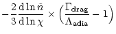
First, we note that the energy equation (Eq. (22)) in the region where drag heating and adiabatic cooling are the dominant terms (which includes the plateau region) can be cast in the simplified form:

 

$$\frac{{\rm d} \ln T}{{\rm d} \ln \chi} -\frac{2}{3} \frac{ {\rm d} \ln \tilde{n}}{ {\rm d} \ln \chi} \times \Big(\frac{\Gamma_{\rm drag}}{\Lambda_{\rm adia}}-1\Big)$$ =

$$\delta^{-1} \times \Big(\frac{G(\chi)}{F(T)}-1\Big),$$ = (24)

where:

 

$$\delta(\chi)^{-1} \equiv \Big(-\frac{2}{3}\frac{{\rm d} \ln \tilde{n}}{{\rm d}\ln\chi}\Big),$$ (25)

remains positive before recollimation and depends only on the MHD solution,

 

$$G(\chi)=-\frac{\frac{1}{c^2} \bigl\Vert \vec{J} \times \vec{B} \b... ...vec{\nabla})\tilde{n}} \propto \frac{M_{\star}^2}{\dot{M}_{{\rm acc}} \varpi_0}$$ (26)

is a positive function, before recollimation, that depends only on the MHD wind solution, and

$$F(T)={kT(1+f_{\rm e})}{\overline{m_{\rm in} f_{\rm i} f_{\rm n} \... ...m in}v\rangle}} \times {\Big( \frac{ \rho }{ \overline{\rho}_{\rm n} } \Big)^2}$$ (27)

also positive, depends only on the local temperature and ionization state of the gas. The functions G and F separate the contributions of the MHD dynamics and ionization processes in the final thermal solution.

Figure 5: Left: function F(T) in erg g cm3 s-1versus temperature assuming local ionization equilibrium and an ionization flux that ionizes only all Na and all C. Center: function $G(\chi )$ in erg g cm3 s-1 for models A, B, C (bottom to top), $\dot M_{\rm acc}= 10^{-6}~M_{\odot}~\rm{yr}^{-1}$ and $\varpi_0=0.1~{\rm AU}$. Right: temperature for model B from the complete calculations in ionization equilibrium (dashed), and assuming $T =T_{\ominus }$ as given by Eq. (30) ( dash-dotted). $\varpi _0=0.1$ AU and accretion rates $\dot{M}_{\rm acc}$ are 10-8 to $10^{-5}~M_{\odot}$ yr-1, from top to bottom.

The function $\delta$ is roughly constant and around unity before recollimation, it diverges at the recollimation point and becomes negative after it. Throughout the plateau  $\delta \sim 1$.

The "wind function'' G is plotted in the center panel of Fig. 5 for our 3 solutions. It rises by 5 orders of magnitude at the wind base and then stabilizes in the jet region (until it diverges to infinity near the recollimation point). The physical reason for its behavior is better seen if we note that the main force driving the flow is the Lorentz force:

$$G\propto \Big\vert\Big\vert\frac{{\rm D}\vec{v}}{{\rm D}t}\Big\vert\Big\vert^2 \times \Big(\frac{{\rm D}\rho}{{\rm D}t}\Big)^{-1}.$$ (28)

For an expanding and accelerating flow $({\rm D}\rho/{\rm D}t)^{-1}$ is an increasing function. At the wind base the Lorentz force accelerates the gas thus causing a fast increase in G. Once the Alfvén point is reached, the acceleration is smaller and ${\rm D}\vec{v}/{\rm D}t$decreases. However this decrease is not so abrupt as in the case of a spherical wind, because the Lorentz force is still at work, both accelerating and collimating the flow. This collimation in turn reduces the rate of increase of $(D\rho/Dt)^{-1}$. The stabilization of G observed after the Alfvén point is thus closely linked to the jet dynamics.

The "ionization function'' F is in general a rising function of Tand is plotted in the left panel of Fig. 5 under the approximation of local ionization equilibrium. Two regimes are present: in the low temperature regime, $f_{\rm i}$  $\gg f_{\rm p}$ is dominated by the abundance of photoionized heavy elements and $F(T) \propto T\,f_{\rm i}$ increases linearly with T, for fixed $f_{\rm i}$. The effect of the UV flux in this region is to shift vertically F(T): for a low UV flux regime only Na is ionized and $f_{{\rm i}} \simeq f(Na{\sc ii})$; for a high UV flux regime were Carbon is fully ionized, $f_{{\rm i}} \simeq f(C{\sc ii})$. In the high temperature regime ( $T \geq 8000$ K) where hydrogen collisional ionization dominates, $f_{\rm i}$ $\simeq f_{\rm p}$, and $F(T) \propto T\,f_{\rm p}$ becomes a steeply rising function of temperature, until hydrogen is fully ionized around $T \simeq 2\times 10^4$ K. The following second rise in F(T) is due to Helium collisional ionization. As we go out of perfect local ionization equilibrium the effect is to decrease the slope of F(T) in the region where H ionization dominates. In the extreme situation of ionization freezing, F(T) becomes linear again as in the photoionized region: $F(T) \propto T f_{{\rm p,freezed}}$.

4.4.2 Conditions needed for a hot plateau

The plateau is simply a region where the temperature does not vary much,

 

$$\frac{{\rm d} \ln T}{{\rm d} \ln \chi} = \epsilon {\hspace{1cm }\rm with \hspace{1cm }} \vert\epsilon\vert\ll 1.$$ (29)

Naively, temperatures $T_\ominus(\chi)$ defined by,

 

$$F(T_\ominus)= G(\chi) \Longleftrightarrow \Gamma_{\rm {drag}} = \Lambda_{\rm {adia}},$$ (30)

will zero the right hand side of Eq. (24) and thus satisfy the plateau condition. This equality is the first constraint on the wind function G, because there must exist a temperature $T_\ominus$ such that the equality holds. However this condition is not sufficient. Indeed the above equality describes a curve $T_\ominus(\chi)$ which must be flat in order to satisfy the plateau condition (Eq. (29)). Therefore the requirement of a flat $T_\ominus$ translates in a second constraint on the variation of G with respect to F. This constraint is obtained by differentiating Eq. (30). We obtain

 

$$\frac{{\rm d} \ln G}{{\rm d} \ln \chi} = \frac{{\rm d} \ln F}{{\rm d} \ln T}\bigg\vert_{T = T_\ominus} \times \epsilon$$ (31)

and after using (Eq. (29)):

$$\Big\vert\Big\vert\frac{{\rm d} \ln G}{{\rm d} \ln \chi}\Big\vert... ...rm d} \ln F}{{\rm d} \ln T} \bigg\vert_{T = T_\ominus}(\chi)\Big\vert\Big\vert.$$ (32)

Thus only winds where the wind function G varies much slower than the ionization function F will produce a plateau. This is fulfilled for our models: below the Alfvén surface, G varies a lot, but collisional H ionization is sufficiently close to ionization equilibrium that F(T) still rises steeply around 10⁴ K (Fig. 5). For our numerical values of G, within our range of $\dot{M}_{\rm acc}$ and $\varpi _0$, we have $T_\ominus \simeq 10^4$ K and thus $\vert{\rm d} \ln G/{\rm d} \ln \chi\vert \ll \vert{\rm d} \ln F/{\rm d} \ln T\vert$. Further out, where ionization is frozen out, we have ${\rm d} \ln F/{\rm d} \ln T = 1$ (because $F\propto T f_{\rm p, freezed}$) but it turns out that in this region G is a slowly varying function of $\chi$, and thus we still have $\vert{\rm d} \ln G/{\rm d} \ln \chi\vert \ll \vert{\rm d} \ln F/{\rm d} \ln T\vert$.

Finally, a third constraint is that the flow must quickly reach the plateau solution $T(\chi) = T_\ominus(\chi)$ and tend to maintain this equilibrium. Let us assume that $T =T_{\ominus }$ is fulfilled at $\chi=\chi_0$, what will be the temperature at $\chi= \chi_0(1+x)$? Letting $T= T_\ominus(1 + \vartheta)$ and assuming $\epsilon \ll 1$, Eq. (24) gives us $\vartheta = \exp(- \alpha x)$, which provides an exponential convergence towards $T =T_{\ominus }$ as long as

$$\alpha= \frac{1}{\delta} \frac{{\rm d} \ln F}{{\rm d} \ln T}\bigg\vert_{T = T_\ominus} > 0 \ .$$ (33)

Note that $\alpha$ depends mainly on the MHD solution (independent of $\dot{M}_{\rm acc}$/$\varpi _0$) and that the steeper the function F, the faster the convergence. The above criterion is always fulfilled in the expanding region of our atomic wind solutions, where $\delta > 0$ and F increases with temperature. The physical reason for the convergence can be easily understood in the following way: it can be readily seen that if at a given point $T> T_\ominus(\chi)$, then $G(\chi)/F(T) < 1$ and the gas will cool (cf. Eq. (24) with $\delta > 0$). Conversely, if $T<T_\ominus(\chi)$, the gas will heat up. Thus, for $\delta > 0$, the fact that F(T) is a rising function introduces a feedback that brings and maintains the temperature close to its local equilibrium value $T_\ominus(\chi)$, and $\Lambda _{\rm adia}$ close to $\Gamma _{\rm drag}$.

We conclude that three analytical criteria must be met by any MHD wind dominated by ambipolar diffusion heating and adiabatic cooling, in order to converge to a hot temperature plateau:
(1) Equilibrium: the wind function G must be such that $F(T)=G(\chi)$ is possible around $T \simeq 10^4$ K;
(2) Small temperature variation: the wind function $G(\chi )$ must vary slower than the ionization function F(T) such that $\vert{\rm d} \ln G/{\rm d} \ln \chi\vert \ll \vert{\rm d} \ln F/{\rm d} \ln T\vert$: (i) the wind must be in ionization equilibrium, or near it, in regions where G is a fast function of $\chi$; (ii) once we have ionization freezing, G must vary slowly, with $\vert {\rm d} \ln G / {\rm d}\ln \chi \vert \ll 1$;
(3) Convergence: $\alpha >0$, i.e. ${2 \over 3} ({\rm d} \ln \tilde{n} / {\rm d} \ln \chi) \times ({\rm d} \ln F / {\rm d} \ln T) \vert_{T = T_\ominus} < 0$, which is always verified for an atomic and expanding wind.

4.4.3 Comments on other MHD winds

Not all types of MHD wind solutions will verify our first criterion. Physically, the large values of $G(\chi )$ observed in our solutions indicates that there is still a non-negligible Lorentz force after the Alfvén surface. In this region (which we call the jet) the Lorentz force is dominated by its poloidal component which both collimates and accelerates the gas (Fig. 1). The gas acceleration translates in a further decrease in density contributing to a further increase in G. Models that provide most of the flow acceleration before the Alfvén surface might turn out to have a lower wind function $G(\chi )$, not numerically compatible with the steep portion of the ionization function F(T). These models would not establish a temperature plateau around 10⁴ K by ambipolar diffusion heating. They would either stabilize on a lower temperature plateau (on the linear part of F(T)) if our second criterion is verified, or continue to cool if G varies too fast for the second criterion to hold. This is the case in particular for the analytical wind models considered by Ruden et al. (1990), where the drag force was computed a posteriori from a prescribed velocity field. The G function for their parameter space (Table 3 of Ruden et al.) peaks at ${\sim}10^{-48}$ erg g cm³ s^-1 at ${\sim} 3~ R_{\star}$ and then rapidly decreases as $G \propto r^{-1}$ for higher radii. This translates into a cooling wind without a plateau.

4.5 Scalings of plateau parameters with $\dot{M}_{acc}$ and $\varpi _0$

Figure 6: Verification of the plateau scalings (Eq. (34)). Left: we plot the measured $T_\ominus f_{{\rm p},\ominus }$ versus $(\dot{M}_{{\rm acc}}\varpi_0)^{-1}$ for all models in out of ionization equilibrium. The evolution is linear except for the very edges of the $(\dot{M}_{{\rm acc}}\varpi_0)^{-1}$ domain. This is due to the failure of our assumptions: in the lower edge $f_{\rm e} < 10^{-4}$ and thus it isn't dominated by H; in the upper edge $f_{\rm e} > 0.1$ and thus the small ionization fraction approximation fails. The crosses are from Safier; because of a smaller momentum transfer rate coefficient they are quite above model C. Right: we plot the measured $f_{{\rm p},\ominus }$ versus $(\dot{M}_{{\rm acc}}\varpi_0)^{-1}$ for Model B in out of ionization equilibrium (solid) and ionization equilibrium (dashed). Note that all the variation is absorbed by $f_{{\rm p},\ominus }$ and thus $f_{{\rm p},\ominus} \propto (\dot{M}_{{\rm acc}}\,\varpi_0)^{-1}$. A straight line is also plot for comparison.

The balance between drag heating and adiabatic cooling (Eq. (30)) can further be used to understand the scalings of the plateau temperature $T_\ominus$ and proton fraction $f_{{\rm p},\ominus }$ with the accretion rate $\dot{M}_{\rm acc}$ and flow line footpoint radius ($\varpi _0$). In the plateau region, ionization is intermediate, i.e., sufficiently high to be dominated by protons but with most of the Hydrogen neutral. Under these conditions we have $F(T)\propto T_{\ominus} f_{{\rm p},\ominus}$. On the other hand, self-similar disk wind models display $G(\chi) \propto (\dot{M}_{{\rm acc}}\varpi_0)^{-1}$ (Eq. (26)). Therefore, we expect

 

$$T_\ominus f_{\rm p} \propto \frac{1} {\dot{M}_{{\rm acc}}\,\varpi_0}\cdot$$ (34)

This behavior is verified in the left panel of Fig. 6 for our out-of-equilibrium results for the 3 wind solutions.

To predict how much of this scaling will be absorbed by $T_\ominus$and how much by $f_{{\rm p},\ominus }$, Safier considered the ionization equilibrium approximation: for the temperature range of the plateau ($T\sim10^4$ K) $f_{\rm p}\simeq$$f_{\rm i}$ is a very fast varying function of T that can be approximated as $f_{\rm p}\propto T^{a}$ with $a \gg 1$. One predicts that $T_{\ominus}\propto (\dot{M}_{{\rm acc}}\,\varpi_0)^{-1/(a+1)}$while $f_{{\rm p},\ominus}\propto (\dot{M}_{{\rm acc}}\,\varpi_0)^{-a/(a+1)} \simeq (\dot{M}_{{\rm acc}}\,\varpi_0)^{-1}$. Hence, the inverse scaling with ( $\dot{M}_{\rm acc}\varpi_0$) should be mostly absorbed by $f_{{\rm p},\ominus }$, while the plateau temperature is only weakly dependent on these parameters. This is verified in the right panel of Fig. 6, where $f_{{\rm p},\ominus }$ in ionization equilibrium is plotted as a function of $(\dot{M}_{{\rm acc}}\,\varpi_0)^{-1}$. The predicted scaling is indeed closely followed.

Let us now turn back to the actual out-of-equilibrium calculations. At the base of the flow we find that the wind evolves roughly in ionization equilibrium (see Fig. 2), however at a certain point the ionization fraction freezes at values that are near those of the ionization equilibrium zone. This effect implies that the ionization fraction should roughly scale as the ionization equilibrium values at the upper wind base. This in indeed observed in Fig. 6. This memory of the ionization equilibrium values by $f_{{\rm p}}$ (as observed in the solar wind by Owocki et al. 1983) is the reason why the scalings of $f_{{\rm p},\ominus }$ with ( $\dot{M}_{\rm acc}\varpi_0$) remain correct. We computed for our solutions the scalings and found for model B: $f_{{\rm p},\ominus}\propto\dot{M}_{{\rm acc}}^{-0.76}$, $f_{{\rm p},\ominus}\propto\varpi_0^{-0.83}$, $T_{\ominus}\propto\dot{M}_{{\rm acc}}^{-0.13}$ and no dependence of T on $\varpi _0$, confirming the memory effect on the ionization fraction only.

Finally, we note that for accretion rates in excess of a few times $10^{-5}~M_{\odot}$  yr^-1, the hot plateau should not be present anymore: Because of its inverse scaling with $\dot{M}_{\rm acc}$, the wind function G remains below 10^-47 erg g cm³ s^-1, and F = G occurs below 10⁴ K, on the linear low-temperature part of F(T) where $f_{{\rm i}} \simeq f(C{\sc ii})$(see Fig. 5). These colder jets will presumably be partly molecular. Interestingly, molecular jets have only been observed so far in embedded protostars with high accretion rates (e.g. Gueth & Guilloteau 1999).

4.6 Effect of the ejection index $\xi$

The importance of the underlying MHD solution is illustrated in Fig. 5. The ejection index $\xi$ is directly linked to the mass loaded in the jet ($\kappa$, see Table 1 and Ferreira 1997). Thus a higher $\xi$ translates in an stronger adiabatic cooling because more mass is being ejected. The ambipolar diffusion heating is less sensitive to the ejection index, because the density increase is balanced by a stronger magnetic field. Hence, the wind function $G(\chi )$ decreases with increasing $\xi$. As a result, the plateau temperature and ionization fraction also decrease (see Eq. (34)).

In Fig. 7 we summarize our results for the three models by plotting the plateau $f_{{\rm p},\ominus }$ versus $T_\ominus$, for several $\dot{M}_{\rm acc}$ (values of $\varpi _0$are connected together). In this plane, our MHD solutions lie in a well-defined "strip'' located below the ionization equilibrium curve, between the two dotted curves. For a given model, as $\dot{M}_{\rm acc}$ increases, the plateau ionization fraction and the temperature both decrease, as expected from the scalings discussed above, moving the model to the lower-left of the strip. Increasing the ejection index decreases $G(\chi )$, and it can be seen that this has a similar effect as increasing $\dot{M}_{\rm acc}$ (Eq. (34)).

Figure 7: Out of ionization equilibrium evolution of wind quantities in the plateau. Points are for all flow lines ( $\varpi _0=0.07\times 1.3^i$ AU and i=0,1,...,10) and accretion rates ( $\dot{M}_{\rm acc}=10^{-i}~M_\odot~{{\rm yr}}^{-1}$ with i=5,6,7,8). We plot, $f_{{\rm p},\ominus }$ versus $T_\ominus$ for all models C (red), B (black), A (blue) and in red the values expected from ionization equilibrium. The dashed/dotted lines are for models without depletion, the solid lines are for models with depletion. The accretion rates increase in the direction top right to bottom left. The thick solid curve traces $f_{{\rm p}}$ in ionization equilibrium, while the two dotted lines embrace the locus of our MHD solutions.

4.7 Depletion effects on the thermal structure

In our calculations we take into account depletion of heavy species into the dust phase. We ran our model with and without depletion and found these effects to be minor. Changes are only found when $f_{{\rm p}} \lesssim 10^{-4}$. The temperature without depletion is slightly reduced (the higher ionization fraction reduces $\Gamma _{\rm drag}$) and as a consequence $f_{{\rm p}}$ is also smaller. Normally these changes affect only the wind base, as the temperature increases $f_{{\rm p}}$ dominates the ionization and we obtain the same results for the plateau zone. However for high accretion rates ( $\dot{M}_{\rm acc}=10^{-5}~M_\odot~{\rm yr}^{-1}$) in the outer wind zone (large $\varpi _0$) we still have $f_{{\rm p}} \lesssim 10^{-4}$ for the plateau and thus the temperature without depletion is reduced there.

  
4.8 Differences with the results of Safier

Figure 8: $\langle\sigma_{\mbox{\tiny H H$^+$ }}v\rangle$ in cm3 s-1 using Draine expression (solid), using Geiss & Buergi expression (see Appendix A.2) (dash) and Draine expression but ignoring the thermal velocity (dot).

The most striking difference between our results and those of Safier is an ionization fraction 10 to 100 times smaller. This difference is mainly due to both different $\langle\sigma_{{\rm H H}^+} v\rangle$ momentum transfer rate coefficients and dynamical MHD wind models.

The critical importance of the momentum transfer rate coefficient ( $\langle\sigma_{{\rm H H}^+} v\rangle$) for the plateau ionization fraction can be seen by repeating the reasoning in the previous section but including the momentum transfer rate coefficient in the scalings. We thus obtain

$$T_\ominus\,f_{{\rm p},\ominus} \propto \frac{1}{\langle\sigma_{{\rm H H}^+} v\rangle \dot{M}_{{\rm acc}} \varpi_0} \cdot$$ (35)

This shows that, because the freezing of the ionization fraction is correlated to the ionization fraction at the base of the wind (which is in ionization equilibrium), $f_{{\rm p}}$ will scale with the momentum transfer rate coefficient value. This means that if the momentum transfer rate coefficient is larger, there is a better coupling between ions and neutrals and hence a smaller drag heating. For the calculation of the $\langle\sigma_{{\rm H H}^+} v\rangle$, Safier ignored the contribution of the thermal velocity in the collisional relative velocity. This considerably reduces $\langle\sigma_{{\rm H H}^+} v\rangle$ and thus, increases $f_{{\rm p}}$. In Fig. 8 we plot the corresponding momentum transfer rate coefficient values. It can be seen that ignoring the thermal contribution to the momentum transfer rate coefficient decreases it typically by a factor of $\gtrsim$6. We also plot in this figure the value obtained by Geiss & Buergi (1986) illustrating the uncertainties in the momentum transfer rate coefficient (more on this in Appendix A.2).