6 Moments expansion

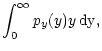
Figure 2: The effective weight $w_{\rm eff}$ can be well approximated using the expansion (66). This plot shows the behavior of the n-th order expansion for a Gaussian weight function with unit variance (see Eq. (75)). The density used, $\rho = 0.5$, corresponds to $\mathcal{N} \simeq 6.3$. The convergence is already extremely good at the second order; for larger values of $\mathcal{N}$ the expansion converges more rapidly.

In the last section we obtained an analytical expansion for Q(s)which has then been used to obtain a first approximation for the correction function C(w) valid for large densities $\rho$. Unfortunately, we have been able to obtain a simple result for C(w)only to first order. Already at the second order, in fact, the correcting function would result in a rather complicated expression involving the error function erf.

Actually, there is a simpler approach to obtain an expansion of C(w)at large $\rho$ using the moments of the random variable y. Given the definition (9) for y, we expect that $\bar y \equiv \langle y \rangle$, the average value of this random variable, increases linearly with the density $\rho$ of objects. Similarly, for large $\rho$ the relative scatter $\bigl\langle (y - \bar y)^2 \bigr\rangle / \bar y^2$ is expected to decrease. In fact, y is the sum of several independent random variables, and thus, in virtue of the central limit theorem, it must converge to a Gaussian random variable with appropriate average and variance.

Since the relative variance of y decreases with $\rho$, we can expand y in the denominator in Eq. (14), obtaining

 

$$C(w) =\rho \int_0^\infty \rm dy \, \frac{p_y(y)}{\bar y + w} \sum... ... (-1)^k \frac{1}{(\bar y + w)^{k+1}} \bigl\langle (y - \bar y)^k \bigr\rangle ,$$ (54)

where we have used the definition of the moments of y:

  

$$\bar y = \langle y \rangle \int_0^\infty p_y(y) y \, \rm dy ,$$ = (55)

$$\bigl\langle (y - \bar y)^k \bigr\rangle \int_0^\infty p_y(y) \bigl( y - \bar y \bigr)^k \, \rm dy .$$ = (56)

In other words, if we are able to evaluate the moments of y we can obtain an expansion of C(w). Actually, the "centered'' moments can be calculated from the "un-centered'' ones, defined by

$$\langle y^k \rangle = \int_0^\infty p_y(y) y^k \, \rm dy = (-1)^k Y^{(k)}(0) .$$ (57)

Here we have used the notation Y^(k)(0) for the k-th derivative of Y(s) evaluated at s = 0. Using Eq. (19) we can explicitly write the first few derivatives

     

Y(0) =1 , (58)

$$\rho Q'(0) ,$$ (59)

$$\rho Q''(0) + \rho^2 \bigl[ Q'(0) \bigr]^2 ,$$ (60)

$$\rho Q'''(0) + 3 \rho^2 Q''(0) Q'(0) + \rho^3 \bigl[ Q'(0) \bigr]^3 ,$$ (61)

$$\rho Q^{(4)}(0) + 4 \rho^2 Q'''(0) Q'(0) + 3 \rho^2 \bigl[ Q''(0) \bigr]^2 + 6 \rho^3 Q''(0) \bigl[ Q'(0) \bigr]^2 + \rho^4 \bigl[ Q'(0) \bigr]^4 .$$ (62)

A nice point here is that, in principle, we can evaluate all the derivatives of Y(s) in terms of derivatives of Q(s) without any technical problem. Moreover, the derivatives of Q(s) in zero are actually directly related to the moments of w. In fact we have

$$Q^{(k)}(0) = (-1)^k \int_\Omega \bigl[w(\vec\theta) \bigr]^k \, \rm d^2 \theta = (-1)^k S_k .$$ (63)

This simple relation allows us to express the moments of y in terms of the moments of w. For the first "centered'' moments we find in particular

  

$$\bar y = \langle y \rangle = \rho , \ \ \bigl\langle (y - \bar y)^2 \bigr\rangle = \rho S_2 ,$$ (64)

$$\bigl\langle (y - \bar y)^3 \bigr\rangle = \rho S_3 , \ \ \bigl\langle (y - \bar y)^4 \bigr\rangle = \rho S_4 + 3 \rho^2 S_2^2 .$$ (65)

Hence, we finally have

 

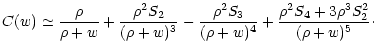
$$C(w) \simeq \frac{\rho}{\rho + w} + \frac{\rho^2 S_2}{(\rho + w)^... ...o^2 S_3}{(\rho + w)^4} + \frac{\rho^2 S_4 + 3 \rho^3 S_2^2}{(\rho + w)^5} \cdot$$ (66)

The first term if this expansion, $\rho / (\rho + w)$, has already been obtained in Eq. (51). Other terms represent higher order corrections to C(w). In Fig. 2 we show the result of applying this expansion to a Gaussian weight.

In closing this section we note that, regardless of the value of $\pi_w$, $P_0 = \rm e^{-\rho \pi_w}$ is vanishing at all orders for $\rho \rightarrow \infty$, and thus we cannot see the peculiarities of finite-support weight functions here.