So far we have considered a finite set ![]() and a fixed number of
objects N. In reality, one often deals with a non-constant number
of objects, so that N is itself a random variable. [For example, if
the objects we are studying are galaxies and if
and a fixed number of
objects N. In reality, one often deals with a non-constant number
of objects, so that N is itself a random variable. [For example, if
the objects we are studying are galaxies and if ![]() is a small
field, the expected number of galaxies in our field will follow a
Poissonian distribution with mean value
is a small
field, the expected number of galaxies in our field will follow a
Poissonian distribution with mean value ![]() ,
where
,
where ![]() is the
density of detectable galaxies in the sky.] Clearly, when we observe
a field
is the
density of detectable galaxies in the sky.] Clearly, when we observe
a field ![]() we will obtain a particular value for the number of
objects N inside the field. However, in order to obtain more
general results, it is convenient to consider an ensemble average, and
take the number of observed objects as a random variable; the results
obtained, thus, will be averaged over all possible values of N.
we will obtain a particular value for the number of
objects N inside the field. However, in order to obtain more
general results, it is convenient to consider an ensemble average, and
take the number of observed objects as a random variable; the results
obtained, thus, will be averaged over all possible values of N.
A way to include the effect of a variable N in our framework is to
note that, although we are observing a small area on the sky, each
object could in principle be located at any position of the whole sky.
Hence, instead of taking N as a random variable and A fixed, we
consider larger and larger areas of the sky and take the limit
![]() .
In doing this, we keep the object density
.
In doing this, we keep the object density
![]() constant. It is easily verified that the two methods (namely
A fixed and N Poissonian random variable with mean
constant. It is easily verified that the two methods (namely
A fixed and N Poissonian random variable with mean ![]() ,
or
rather
,
or
rather
![]() with
with
![]() fixed), lead to the
same results. In the following, however, we will take the latter
scheme, and let A go to infinity; correspondingly we take
fixed), lead to the
same results. In the following, however, we will take the latter
scheme, and let A go to infinity; correspondingly we take ![]() as the whole plane.
as the whole plane.
From Eq. (16) we see that W(s) is proportional to 1/A.
For this reason it is convenient to define the function
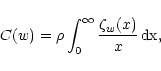
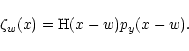
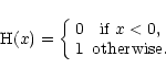
In order to further simplify the expression for the correcting factor
C(w), we rewrite its definition as
Copyright ESO 2001
![\begin{displaymath}
Q(s) = \int_\Omega \left[ \rm e^{-s w(\vec\theta)} - 1 \right] \,
\rm d^2 \theta .
\end{displaymath}](/articles/aa/full/2001/25/aa1052/img68.gif)
![\begin{displaymath}
Y(s) = \lim_{N \rightarrow \infty} \left[ 1 + \frac{Q(s) \rho}{N}
\right]^{N-1} = \rm e^{\rho Q(s)} .
\end{displaymath}](/articles/aa/full/2001/25/aa1052/img69.gif)
 = \rm e^{-ws} Y(s) .
\end{displaymath}](/articles/aa/full/2001/25/aa1052/img75.gif)
 = \int_s^\infty Z_w(s') \, \rm ds'
,
\end{displaymath}](/articles/aa/full/2001/25/aa1052/img77.gif)
 = \rho
\int_...
...s' =\rho \int_0^\infty \rm e^{-w s'} Y(s') \, \rm ds' = \mathcal L[\rho
Y](w) .$](/articles/aa/full/2001/25/aa1052/img78.gif)