

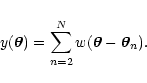
Up: Smooth maps from clumpy
2 Definitions and first results
Suppose one wants to measure an unknown field
 ,
a
function of the "position''
,
a
function of the "position''
 .
[What
really
means is totally irrelevant for our discussion. For example,
could represent the position of an object on the sky, the
time of some observation, or the wavelength of a spectral feature. In
the following, to focus on a specific case, we will assume that
represents a position on the sky and thus we will
consider it as a two-dimensional variable.] Suppose also that we can
obtain a total of N unbiased estimates
.
[What
really
means is totally irrelevant for our discussion. For example,
could represent the position of an object on the sky, the
time of some observation, or the wavelength of a spectral feature. In
the following, to focus on a specific case, we will assume that
represents a position on the sky and thus we will
consider it as a two-dimensional variable.] Suppose also that we can
obtain a total of N unbiased estimates  for fat some points
 ,
and that each point can
freely span a field
,
and that each point can
freely span a field  of surface A (
represents the
area of the survey, i.e. the area where data are available). The
points
,
in other words, are taken to be
independent random variables with a uniform probability
distribution and density
of surface A (
represents the
area of the survey, i.e. the area where data are available). The
points
,
in other words, are taken to be
independent random variables with a uniform probability
distribution and density
 inside the set
of
their possible values. We can then define the smooth map of
Eq. (1), or more explicitly
inside the set
of
their possible values. We can then define the smooth map of
Eq. (1), or more explicitly
 |
(5) |
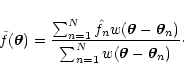
In the rest of this paper we study the expectation value
 of
of
 (an
alternative weighting scheme is briefly discussed in
Appendix A). To simplify the notation we
will assume, without loss of generality, that the weight function
(an
alternative weighting scheme is briefly discussed in
Appendix A). To simplify the notation we
will assume, without loss of generality, that the weight function
 is normalized, i.e.
 |
(6) |
In order to obtain the ensemble average of  we need to
average over all possible measurements at each point, i.e. ,
and over all possible positions
for the N points. The first average is trivial, since
is linear on the data
and the data are
unbiased, so that
we need to
average over all possible measurements at each point, i.e. ,
and over all possible positions
for the N points. The first average is trivial, since
is linear on the data
and the data are
unbiased, so that
 .
We then have
.
We then have
 = =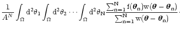 |
(7) |
Relabeling the integration variables we can rewrite this expression as
=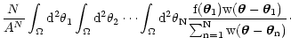 |
(8) |
We now define a new random variable
 |
(9) |
Note that the sum runs from n=2 to n=N. Let us call py(y) the
probability distribution for
 .
If we suppose that
is not close to the boundary of ,
so that the
support of
.
If we suppose that
is not close to the boundary of ,
so that the
support of
 (i.e. the set of points
 where
where
 )
is inside
,
then the probability distribution for
does
not depend on
.
We anticipate here that below we will
take the limit of large surveys, so that
tends to the whole
plane, and
)
is inside
,
then the probability distribution for
does
not depend on
.
We anticipate here that below we will
take the limit of large surveys, so that
tends to the whole
plane, and
 ,
,
 ,
such that
remains constant. Since, by definition, the weight
function is assumed to be non-negative, py(y) vanishes for y < 0.
Analogously, we call pw(w) the probability distribution for the
weight w. These two probability distributions can be calculated
from the equations
,
such that
remains constant. Since, by definition, the weight
function is assumed to be non-negative, py(y) vanishes for y < 0.
Analogously, we call pw(w) the probability distribution for the
weight w. These two probability distributions can be calculated
from the equations
pw(w) =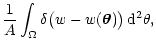 |
(10) |
py(y)=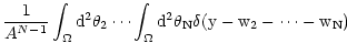 = =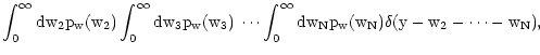 |
(11) |
where  is Dirac's distribution and where we have called
 .
Note that Eqs. (10) and (11) hold
only if the N points
are uniformly
distributed on the area A with density
.
Note that Eqs. (10) and (11) hold
only if the N points
are uniformly
distributed on the area A with density  ,
and if there is no
correlation (so that the probability distribution for each point is
,
and if there is no
correlation (so that the probability distribution for each point is
 ). Moreover, we are assuming here
that the probability distribution for
does not depend
on
.
This is true only if a given configuration of points
has the same probability as the
translated set
). Moreover, we are assuming here
that the probability distribution for
does not depend
on
.
This is true only if a given configuration of points
has the same probability as the
translated set
 .
This
translation invariance, clearly, cannot hold exactly for finite fields
;
on the other hand, again, as long as
is far
from the boundary of the field, the probability distribution for
is basically independent of
.
Note that
in the case of a field with masks, we also have to exclude in our
analysis points close to the masks.
.
This
translation invariance, clearly, cannot hold exactly for finite fields
;
on the other hand, again, as long as
is far
from the boundary of the field, the probability distribution for
is basically independent of
.
Note that
in the case of a field with masks, we also have to exclude in our
analysis points close to the masks.
Using py we can rewrite Eq. (8) in a more compact form:
=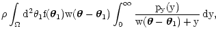 |
(12) |
where, we recall,
is the density of objects. For the
following calculations, it is useful to write this equation as
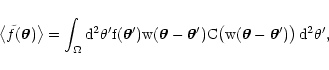 |
(13) |
where C(w) the correcting factor, defined as
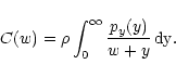 |
(14) |
Finally, we will often call the combination
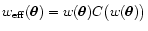 ,
which enters Eq. (13), effective weight.
,
which enters Eq. (13), effective weight.
Interestingly, Eq. (13) shows that the relationship between
and
is a simple convolution with the kernel
 .
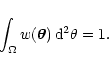
From the
definition (5), we can also see that this kernel is
normalized, in the sense that
.
From the
definition (5), we can also see that this kernel is
normalized, in the sense that
 |
(15) |
In fact, if we consider a "flat'' signal, for instance
 ,
we clearly obtain
,
we clearly obtain
 .
On the other hand, from the properties of
convolutions, we know that the ratio between the l.h.s. and the
r.h.s. of Eq. (15) is constant, independent of the function
.
We thus deduce that this ratio is 1, i.e. that
Eq. (15) holds in general. The normalization of
will be also proved below in
Sect. 5.1 using analytical techniques.
.
On the other hand, from the properties of
convolutions, we know that the ratio between the l.h.s. and the
r.h.s. of Eq. (15) is constant, independent of the function
.
We thus deduce that this ratio is 1, i.e. that
Eq. (15) holds in general. The normalization of
will be also proved below in
Sect. 5.1 using analytical techniques.
If py(y) is available, Eq. (12) can be used to obtain the
expectation value for the smoothed map .
In order to obtain
an expression for py we use Markov's method (see, e.g.,
Chandrasekhar 1943; see also Deguchi & Watson 1987 for an application
to microlensing studies). Let us define the Laplace transforms of
py and pw:
W(s)= = \int_0^\infty \rm e^{-sw} p_w(w) \, \rm dw
=\frac{1}{A} \int_\Omega \rm e^{-sw(\vec\theta)} \, \rm d^2
\theta ,$](/articles/aa/full/2001/25/aa1052/img64.gif) |
(16) |
Y(s)= = \int_0^\infty \rm e^{-sy} p_y(y) \, \rm dy
= \bigl[ W(s) \bigr]^{N-1} .$](/articles/aa/full/2001/25/aa1052/img65.gif) |
(17) |
Hence py can in principle be obtained from the following scheme.
First, we evaluate W(s) using Eq. (16), then we calculate
Y(s) from Eq. (17), and finally we back-transform this
function to obtain py(y).
Up: Smooth maps from clumpy
Copyright ESO 2001