7 Examples

In this section we consider three typical examples of weight functions, namely a top-hat function, a Gaussian, and a parabolic weight function. For simplicity, in the following we will consider weight functions with fixed "width''. The results obtained can then be adapted to weight functions with different widths using the scaling property (Sect. 5.2).

   
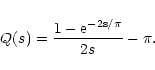
7.1 Top-hat

The simplest case we can consider for $w(\vec\theta)$ is a top-hat function of unit radius, which can be written as

$$w(\vec\theta) = \frac{1}{\pi} {\rm H}\bigl( 1 - \vert \vec\theta \vert \bigr) .$$ (67)

In this case we immediately find for w > 0

  

$$\pi \bigl( \rm e^{-s/\pi} - 1 \bigr) ,$$ (68)

$$\exp \bigl[ \pi\rho \bigl( \rm e^{-s/\pi} - 1 \bigr) \bigr] .$$ (69)

We now note that since $w(\vec\theta)$ is either 0 or $1/\pi$, we just need to evaluate $C(1/\pi)$. We then find

$$C(1/\pi) = \frac{\rho}{1 - P_0} \int_0^\infty \rm e^{-s/\pi} Y(s) \, \rm ds = 1 ,$$ (70)

as expected.

For the top-hat function we can also explicitly obtain the probability distribution for y. If w > 0 we have

$$p_y(y) = \sum_{n = 0}^\infty \frac{\rm e^{-\rho \pi} (\rho \pi)^n}{\pi n!} \delta(y - n/\pi) ,$$ (71)

and thus

 

$$C(w) =\frac{\rho}{1 - P_0} \int_0^\infty \frac{p_y(y)}{w + y} \, ... ...P_0}{\pi (1 - P_0)} \sum_{n=0}^\infty \frac{(\rho \pi)^n}{(w + n/\pi) n!} \cdot$$ (72)

From this expression we easily obtain $C(1/\pi) = 1$. Moreover, we can evaluate the two limits

  

$$\lim_{w \rightarrow \infty} w C(w) \frac{\rho}{1 - P_0} ,$$ = (73)

$$\lim_{w \rightarrow 0^+} w C(w) \frac{\rho P_0}{1 - P_0} ,$$ = (74)

thus regaining the results of Sect. 5.3.

   
7.2 Gaussian

Figure 3: Effective weight function corresponding to a Gaussian weight function. The original weight function is a normalized Gaussian of unit variance, with weight area $\mathcal{A} \simeq 12.5$. Significantly broader effective weights are obtained if the weight number is smaller than $\mathcal{N} < 10$.

A weight function commonly used is a Gaussian of the form

$$w(\vec\theta) = \frac{1}{2 \pi} \exp\bigl( - \vert \vec\theta \vert^2 / 2 \bigr) .$$ (75)

Unfortunately, we cannot explicitly integrate Q(s) and thus we are unable to obtain a finite expression for C(w). The results of a numerical calculations are however shown in Fig. 3.

   
7.3 Parabolic weight

Figure 4: Effective weight function corresponding to a Gaussian weight function. Note the discontinuity at $\vert \vec\theta \vert = 1$, corresponding to the boundary of the support of w. The original weight function is a normalized parabolic function with weight area $\mathcal{A} \simeq 2.4$. Note that this weight area is significantly smaller than the ones encountered in previous examples. For low densities, $w_{\rm eff}$ converges to a top-hat function, in accordance with the results of Sect. 5.4.

As the last, example we consider a parabolic weight function with expression

$$w(\vec\theta) = \left\{ \begin{array}{cc} \frac{2}{\pi} ... ... < 1 ,$ } \\ 0 & \textrm{otherwise$ .$ } \end{array}\right.$$ (76)

We then find

$$Q(s) = \frac{1 - \rm e^{-2s/\pi}}{2 s} - \pi .$$ (77)

Unfortunately, we cannot proceed analytically and determine C(w). We thus report the results of numerical integrations in Fig. 4. Note that, as expected, the resulting effective weight has a discontinuity at $\vert \vec\theta \vert = 1$.