A&A 431, 729-746 (2005)
DOI: 10.1051/0004-6361:20041737

Multiple solutions for asteroid orbits: Computational procedure and applications

A. Milani¹ - M. E. Sansaturio² - G. Tommei¹ - O. Arratia² - S. R. Chesley³

1 - Dipartimento di Matematica, Università di Pisa, via Buonarroti 2, 56127 Pisa, Italy
2 - E.T.S. de Ingenieros Industriales, University of Valladolid Paseo del Cauce 47011 Valladolid, Spain
3 - Jet Propulsion Laboratory, 4800 Oak Grove Drive, CA-91109 Pasadena, USA

Received 27 July 2004 / Accepted 20 October 2004

Abstract
We describe the Multiple Solutions Method, a one-dimensional sampling of the six-dimensional orbital confidence region that is widely applicable in the field of asteroid orbit determination. In many situations there is one predominant direction of uncertainty in an orbit determination or orbital prediction, i.e., a "weak'' direction. The idea is to record Multiple Solutions by following this, typically curved, weak direction, or Line Of Variations (LOV). In this paper we describe the method and give new insights into the mathematics behind this tool. We pay particular attention to the problem of how to ensure that the coordinate systems are properly scaled so that the weak direction really reflects the intrinsic direction of greatest uncertainty. We also describe how the multiple solutions can be used even in the absence of a nominal orbit solution, which substantially broadens the realm of applications. There are numerous applications for multiple solutions; we discuss a few problems in asteroid orbit determination and prediction where we have had good success with the method. In particular, we show that multiple solutions can be used effectively for potential impact monitoring, preliminary orbit determination, asteroid identification, and for the recovery of lost asteroids.

Key words: minor planets, asteroids - celestial mechanics - astrometry - surveys

1 Introduction

When an asteroid has just been discovered, its orbit is weakly constrained by observations spanning only a short arc. Although in many cases a nominal orbital solution (corresponding to the least squares principle) exists, other orbits are acceptable as solutions, in that they correspond to rms of the residuals not significantly above the minimum. We can describe this situation by defining a confidence region $Z(\chi)$ in the orbital elements space such that initial orbital elements belong to $Z(\chi)$ if the penalty (increase in the target function, essentially the sum of squares of the residuals, with respect to the minimum) does not exceed some threshold depending upon the parameter $\chi$. This situation also has a probabilistic interpretation, in that the probability density at a given set of initial orbital elements is a decreasing function of the penalty.

The problem is that in many applications we need to consider the set of the orbits with initial conditions in the confidence region as a whole. For example, we may need to predict some future (or past) event such as an observation, the values of the perturbed orbital elements, a close approach or even an impact, and this for all "possible'' orbits, i.e., for every solution resulting in acceptable residuals. Since the dynamic model for asteroid orbits, essentially the N-body problem, is not integrable there is no way to compute all the solutions for some time span in the future (or past). We can only compute a finite number of orbits by numerical integration.

Thus we must introduce the concept of the Virtual Asteroid (VA). The confidence region is sampled by a finite number of VAs, each one with an initial condition in the confidence region; in practice, the number of VAs can range between few tens and few tens of thousands, depending upon the application and upon the available computing power. This abstract definition, however, does not indicate how a finite number of VAs are selected among the continuum set of orbital elements spanning the confidence region. It is perfectly acceptable to select the VAs at random in the confidence region: this is the heart of the so called Monte Carlo methods. The question arises if there is some method to select the VAs which is optimal, in the sense of representing the confidence region with a minimum number of points, thus with the minimum computational load for whatever prediction.

The above question does not have a unique answer because, of course, it depends upon the nature and the time of the prediction to be computed. However, there is a basic property of the solutions of the N-body problem which helps in suggesting an answer appropriate in many cases. Whatever the cloud of VAs selected, unless they all have the same semimajor axis, as time goes by the orbits will spread mostly along track because of their different periods. Thus, after a long enough time, the set of VAs will appear as a necklace, with pearls spread more or less uniformly along a wire which is not very different from a segment of a heliocentric ellipse. When this segment is long, e.g., a good fraction of the entire length of the ellipse, the distance along track to the VA nearest the one being considered controls the resolution of the set of predictions obtained by computing all the VA orbits. Then it is clear that maximum efficiency is obtained by spreading the VAs as uniformly as possible along the necklace.

Thus the basic idea of our method can be described as follows. We will select a string, that is a one-dimensional segment of a (curved) line in the initial conditions space, the Line Of Variations (LOV). There is a number of different ways to define, and to practically compute, the LOV, but the general idea is that a segment of this line is a kind of spine of the confidence region. Note that a simpler and more approximate notion of LOV has been in use for a long time; it was obtained by fixing the value of all the orbital elements (e.g., to the values corresponding to the nominal solution), and by changing only the mean anomaly. When, after a long time span, small differences in semimajor axis have propagated into significant along track differences, this is indeed an approximation of the LOV (as defined here) good enough to be useful in many cases, but not always.

Several different definitions of the LOV are possible. Milani (1999) proposed a definition of the LOV as the solution of an ordinary differential equation, with the nominal least squares solution as initial condition and the vector field defined by the weak direction of the covariance matrix. However, in the same paper it was pointed out that such differential equation is unstable, in particular in the cases where there is a largely dominant weak direction, the same cases in which the definition of the LOV is most useful. Thus a corrective step was introduced, based upon differential corrections constrained on the hyperplane perpendicular to the weak direction. This provided a stable algorithm to compute an approximation of the LOV as defined in that paper.

In this paper we show that the constrained differential corrections algorithm can be used to define the LOV as the set of points of convergence. By adopting this alternate definition we have two advantages. First, we have a definition exactly (not approximately) corresponding to the numerically effective algorithm used to compute the sample points along the LOV. Second, this new definition does not use the nominal solution as an initial condition, thus it is possible to define, and to practically compute, the LOV even when the nominal least squares solution either does not exist or anyway has not been found.

That is, the constrained differential corrections algorithm can provide one solution along the LOV, starting from some initial guess (which a posteriori may prove to be very far from the real orbit). This procedure can be conceived as an intermediate step between the preliminary orbit and the full differential corrections, and thus used to increase the number of final least squares solutions. Even when the full differential corrections fail, the constrained solution can be used to compute ephemerides of the object, to be used for short term recovery. In both the above uses, the constrained solution can play a role similar to the one of the so called Väisälä orbits.

Once the LOV is defined, it is quite natural to sample it by VAs at regular intervals in the variable which is used to parameterize the curve. Depending upon which definition is used, there is a natural parameterization. If the LOV is defined as solution of a differential equation, the natural parameter is the independent variable of the differential equation. If it is defined as set of points of convergence of a constrained differential corrections, a parameter related to the $\chi^2$ of the fit could be used. However, if the definition is generalized to the case where the nominal solution is not available, there is no natural way to assign the value zero of the parameter to one specific solution.

Anyway, once the sample is selected with equal spacing on the LOV, if the time span between initial conditions and prediction is long, but there are no strong perturbations in between, then the VAs will remain approximately uniformly spaced in the necklace. When there are close approaches in between discovery and prediction time the situation can become much more complicated (Milani et al. 2004b), but still the sampling is more efficient than a Monte Carlo one.

This idea of "multiple solutions'' sampling of the LOV was introduced by Milani (1999) and used in different applications, such as recovery of lost asteroids (Boattini et al. 2001) and identification of possible impacts (Milani et al. 1999). In this paper we discuss additional applications, including asteroid identification and a more advanced form of impact monitoring.

With the alternate definition introduced in this paper, the same applications become possible also in the case in which the nominal solution is not available, e.g., because of divergence of the differential correction process (as it is often the case when the observations are few or only cover a short time span). In this case the LOV is defined, but we do not have the nominal solution to act as a reference point on the LOV. Nevertheless, the multiple solutions along the LOV can be used, e.g., in identifications. This is especially important because the asteroids for which a nominal solution cannot be computed are the ones which would be considered lost according to the conventional algorithms. Each case in which the new algorithms, discussed in this paper (and also in another paper in preparation), allow us to find other observations for a lost asteroid has to be considered a success of comparable importance to the discovery of a new object, because it is indeed a rediscovery.

The LOV can be also used as a tool to explore the geometry of the confidence region, and this is of course more useful when this geometry is complicated. When the penalty has separate local minima, the confidence regions $Z(\chi)$ can have a topology changing with the value of $\chi$, that is, the number of connected components can change. This phenomenon is already known in the context of preliminary orbit determination: the Gauss problem of a two-body ellipse satisfying three observations can have multiple solutions. For asteroids observed only over a short arc, especially if this occurs near quadrature, it is possible to have a sum of squares of the residuals with several local minima, each one close to one of the Gauss solutions. Exploring the full geometry of the confidence region in these cases is very difficult, but the behavior of the sum of squares along the LOV can provide enough information to understand the situation, and to avoid the faulty predictions which could result from a simplistic approach.

2 The line of variations

 To discuss the definitions of the Line Of Variations we need to recall some known results and define some notation about the least squares orbit determination procedure.

2.1 Newton's method and differential corrections

The weighted least squares method of orbit determination seeks to minimize the weighted rms of the m observation residuals $\Xi=(\xi_i),\; i=1,\ldots,m$, so we define the cost function

$$Q=\frac{1}{m}\;\Xi^T W~ \Xi ,$$

where W is a square, symmetric, positive-definite $m\times m$ matrix that should reflect the a priori rms and correlations of the observation errors. We denote the design matrix, with the partials of the residuals with respect to the elements by

$$B=\frac{\partial \Xi}{\partial X}~(X) ,$$

an $m\times 6$ matrix. Then we can compute the gradient of the cost function

$$\frac{\partial Q}{\partial X}={2 \over m}\; \Xi ^T W~ B .$$

The stationary points of the cost function Q are solutions of the system of nonlinear equations $\partial Q/\partial X=0$, which are usually solved by some iterative procedure. The standard Newton's method involves the computation of the second derivatives of the cost function:

$$\frac{\partial^2 Q}{\partial X^2}= {2 \over m} \left[ B^T W~ ... ...~W~ \frac{\partial B}{\partial X}\right]= {2 \over m} \; C^N ,$$

where C^N is a $6\times 6$ matrix, positive definite in the neighborhood of a local minimum. Then one iteration of Newton's method provides a correction $X \longrightarrow X+\Delta X$ with

$$\Delta X= \left[ C^N\right]^{-1} D ,$$

where

$$D=-B^T W \Xi = -{m\over 2} \frac{\partial Q}{\partial X}^T \cdot$$

However, the most used method is a variant of Newton's method, known in this context as differential corrections, with each iteration making the correction

$$\Delta X = -(B^T W B)^{-1}B^T W \Xi .$$

Thus the difference between Newton's method and the differential corrections method is only in the use of the normal matrix C=B^T W B instead of the matrix C^N, and the covariance matrix $\Gamma=C^{-1}$ instead of $\Gamma_N=[C^N]^{-1}$; note that the right hand side D of the normal equations is the same. One motivation for this simplification is that the computation of the three-index arrays of second derivatives $\partial B/\partial X=\partial^2 \Xi/\partial X^2$ requires to solve 216 scalar differential equations (on top of the usual 6+36 for the equations of motion and the variational equations for the first derivatives).

With both methods, if the iterative procedure converges, the limit X^* is a stationary point of the cost as a function of the elements X, that is $D(X^*)=\underline 0$. If a stationary point X^* is a local minimum of Q(X) it is called a best-fitting or nominal solution. Such nominal solutions may not be unique (see Sect. 6), although they are generally unique when there are enough observations over a long enough span of time.

There are cases of orbit determination with stationary points of Q(X) not corresponding to local minima, but to generalized saddles (Sansaturio et al. 1996); thus the matrix C^N, proportional to the Hessian matrix, has some negative eigenvalue. Since C can have only eigenvalues $\geq 0$, the saddles need to correspond to cases in which the term $\Xi~W~{\partial B}/{\partial X}$ provides a significant contribution to C^N, to the point of changing the sign of at least one eigenvalue. This can happen more easily when the residuals $\Xi$are large, that is the saddle corresponds to a value of Q well above the minimum. However, if the matrix C is badly conditioned, a very small eigenvalue of C can be perturbed into a negative eigenvalue of C^N even with moderate residuals $\Xi$, as in the example in Sect. 6.

The expansion of the cost function at a point $X = X^* + \Delta X$ in a neighborhood of X^* is

$$Q(X^*) +\frac{1}{m} ~\Delta X^T~ C^N~\Delta X + \ldots$$                            Q(X) =

$$Q(X^*) +\frac{1}{m} ~\Delta X^T~ C~\Delta X + \ldots = Q(X^*)+\Delta Q(X) ,$$ =

where the dots in the first equality indicate terms of order $\geq$3 in $\Delta X$, the dots in the second line contain also a term with the second derivative of $\Xi$, which is only second order in $\Delta X$, although it contains also $\Xi$. A confidence region $Z(\chi)$is defined by setting an upper limit to the penalty $\Delta Q$:

$$Z(\chi)=\left\{X\;\vert\; \Delta Q(X) \leq \chi^2/m\right\} .$$

2.2 The ellipsoid approximation

If the confidence region is small and the residuals are small, then all the higher order terms in the cost function are negligible and the confidence region is well approximated by the confidence ellipsoid $Z_{\rm L}(\chi)$ defined by the quadratic inequality

$$Z_{\rm L}(\chi)=\left\{X\;\vert\; \Delta X^T~ C(X^*)~\Delta X \leq \chi^2\right\} .$$

Let the longest semiaxis of the confidence ellipsoid be in the direction of the unit vector V₁, which is an eigenvector of the normal matrix C(X^*), computed at the nominal solution:

$$C(X^*)~ V_1= \lambda_1 V_1$$

and the eigenvalue $\lambda_1$ is the smallest among the eigenvalues of C(X^*); the longest semiaxis of the confidence ellipsoid $Z_{\rm L}(1)$ has length $k_1=1/\sqrt{\lambda_1}$. Note that V₁ is also an eigenvector of  $\Gamma(X^*)$ with eigenvalue $1/\lambda_1=k_1^2$.

Let H be the hyperplane spanned by the other eigenvectors $V_j, j=2,\ldots,6$. The tip of the longest axis of the confidence ellipsoid $X_1=X^* + k_1\;V_1$ has the property of being the point of minimum of the cost function restricted to the affine space X₁+H. It is also the point of minimum of the cost function restricted to the sphere $\vert\Delta X\vert=k_1$. These properties, equivalent in the linear regime, are not equivalent in general (see Appendix A).

2.3 The weak direction vector field

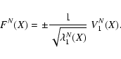
Let us consider the vector k₁(X) V₁(X). Indeed such vector can be defined at every point of the space of initial conditions X: the normal matrix C(X) is defined everywhere, thus we can find at each point X the smallest eigenvalue of C(X):

$$C(X)~V_1(X)= \lambda_1(X)\;V_1(X) = \frac 1{k_1^2(X) } \; V_1(X)$$

and the product $k_1(X)\;V_1(X)$ is a vector field defined for every X.

The unit eigenvector V₁ is not uniquely defined, of course -V₁is also a unit eigenvector. Thus $k_1(X)\;V_1(X)$ is what is called an axial vector, with well defined length and direction but undefined sign. However, given an axial vector field defined over a simply connected set, there is always a way to define a true vector field F(X) such that the function $X \mapsto F(X)$ is continuous. At the beginning of the procedure we can select the sign according to some rule, e.g., in such a way that the directional derivative of the semimajor axis a is positive in the direction +V₁(X), or that the heliocentric distance is increasing. Then the consistency of the orientation is maintained by continuation.

Other problems could arise if the normal matrix C(X), for some value of the initial condition X, had a smallest eigenvalue of multiplicity 2. The exact equality of two eigenvalues does not occur generically, and even an approximate equality is rare, as it is possible to check with a large set of examples. Anyway, whenever the two smallest eigenvalues are of the same order of magnitude the LOV method has serious limitations, as discussed in Sect. 2.6.

Given the vector field F(X) as defined above, the differential equation

$$\frac{{\rm d}X}{{\rm d}\sigma}= F(X)$$

has a unique solution for each initial condition, because the vector field is smooth. Let us select the initial condition X(0)=X^*, that is $\sigma=0$ corresponds to the nominal solution. Then there is a unique solution $X(\sigma)$.

In the linear approximation, the solution $X(\sigma)$ is the tip of the major axis of the confidence ellipse $Z_{\rm L}(\sigma)$. When the linear approximation does not apply, $X(\sigma)$ is indeed curved and can be computed only by numerical integration of the differential equation.

This approach was used to define the LOV in Milani (1999). However, such a definition has the handicap of numerical instability in the algorithms to compute it. As an intuitive analogy, for weakly determined orbits the graph of the cost function is like a very steep valley with an almost flat river bed at the bottom. The river valley is steeper than any canyon you can find on Earth; so steep that the smallest deviation from the stream line sends you up the valley slopes by a great deal. This problem cannot be efficiently solved by brute force, that is by increasing the order or decreasing the stepsize in the numerical integration of the differential equation. The only way is to slide down the steepest slopes until the river bed is reached again, which is the intuitive analog of the new definition.

   
2.4 The constrained differential corrections

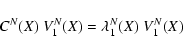
If the axial vector field V₁(X) is defined for all X, then the orthogonal hyperplane H(X) is also defined:

$$H(X)=\{ Y \vert (Y-X)\cdot V_1(X)=0\} .$$

Given an initial guess X, it is possible to compute a differential correction constrained to H(X) by defining the $5\times m$ matrix B_H(X) with the partial derivatives of the residuals with respect to the coordinates of the vector H on H(X). Then the constrained normal equations are defined by the constrained normal matrix C_H, which gives the restriction of the linear map associated to C to the hyperplane H(X), and by the right hand side D_H, which is the component of vector D along the hyperplane:

$$C_H=B_H^T W~ B_H ;\quad D_H=-B_H^T W ~ \Xi ;\quad C_H \Delta H = D_H$$

with solution

$$\Delta H= \Gamma_H \; D_H ;\quad\Gamma_H= C_H^{-1}$$

where the constrained covariance matrix $\Gamma_H$ is not the restriction of the covariance matrix $\Gamma$ to the hyperplane (cf. Milani 1999, Sect. 2.3). The computation of C_H, D_H can be performed by means of a rotation to a new basis in which V₁(X) is the first vector, then C_H is obtained by removing the first row and the first column of C, D_H by removing the first coordinate from D.

The constrained differential correction process is obtained by computing the corrected $X'=X+\Delta X$ where $\Delta X$ coincides with $\Delta H$ along H(X) and has zero component along V₁(X). Then the weak direction and the hyperplane are recomputed: V₁(X'), H(X') and the next correction is constrained to H(X'). This procedure is iterated until convergence. If $\overline X$ is the convergence value, then $D_H(\overline X)=\underline 0$, that is the right hand side of the unconstrained normal equation is parallel to the weak direction

$$D(\overline X)\;\vert\vert\; V_1(\overline X) .$$

The above equation is equivalent to the following property: the restriction of the cost function to the hyperplane $H(\overline X)$ has a stationary point in $\overline X$: the constrained corrections correspond to the intuitive idea of "falling down to the river''.

Thus we can introduce a new definition of LOV as the set of points X such that D(X)||V₁(X) (the gradient of the cost function is in the weak direction). If there is a nominal solution X^*, then D(X^*)=0, thus it belongs to the LOV. However, the LOV is defined independently from the existence of a local minimum of the cost function.

   
2.5 Parameterizing and sampling the LOV

The equation D(X)||V₁(X) corresponds to five scalar equations in six unknowns, thus it has generically a smooth one parameter set of solutions, i.e., a differentiable curve. However, we do know an analytic or anyway direct algorithm neither to compute the points of this curve nor to find some natural parameterization (e.g., by the arclength).

An algorithm to compute the LOV by continuation from one of its points X is the following. The vector field F(X), deduced from the weak direction vector field V₁(X), is orthogonal to H(X). A step in the direction of F(X), such as an Euler step of the solution of the differential equation ${\rm d}X/{\rm d}\sigma=F(X)$, that is $X'=X+\delta\sigma\;F(X)$, is not providing another point on the LOV, unless the LOV itself is a straight line (see Appendix A); this would be true even if the step along the solutions of the differential equation is done with a higher order numerical integration method, such as a Runge-Kutta. However, X' will be close to another point X'' on the LOV, which can be obtained by applying the constrained differential corrections algorithm, starting from X' and iterating until convergence.

If X was parameterized as $X(\sigma)$, we can parameterize $X''=X(\sigma+\delta\sigma)$, which is an approximation since the value $\sigma+\delta\sigma$ actually pertains to X'. As an alternative, if we already know the nominal solution X^* and the corresponding local minimum value of the cost function Q(X^*), we can compute the $\chi$ parameter as a function of the value of the cost function at X'':

$$\chi=\sqrt{m\cdot [Q(X'')-Q(X^*)]} .$$

In the linear regime, the two definitions are related by $\sigma=\pm\chi$, but this is by no means the case in strongly nonlinear conditions. Thus we can adopt the definition $\sigma_Q=\pm \chi$, where the sign is taken to be the same as that of $\sigma$, for an alternate parameterization of the LOV.

If we assume that the probability density at the initial conditions X is an exponentially decreasing function of $\chi$, as in the classical Gaussian theory (Gauss 1809), then it is logical to terminate the sampling of the LOV at some value of $\chi$, that is, the LOV we are considering is the intersection of the solution of the differential equation with the nonlinear confidence region Z(b). When $\chi=\vert\sigma_Q\vert>b$ we stop sampling, even if $\vert\sigma\vert<b$.

The algorithm described above can actually be used in two cases: a) when a nominal solution is known, and b) when it is unknown, even nonexistent. If the nominal solution X^* is known, then we set it as the origin of the parameterization, X^*=X(0) and proceed by using either $\sigma$ or $\sigma_Q$ as parameters for the other points computed with the alternating sequence of numerical integration steps and constrained differential corrections. If, on the other hand, a nominal solution is not available we must first reach some point on the LOV by making constrained differential corrections starting from some potentially arbitrary initial condition (see Sect. 4.1). Once on the LOV we can begin navigating along it in the same manner as is done when starting from the nominal point.

Table 1: Description of the five element sets used in the computations of the LOV, and their respective native units and rescaling parameters.

In such cases, we set the LOV origin X(0) to whichever point $\overline X$ of the LOV we have first found with constrained differential corrections, when starting from the initial guess. We then compute the other points as above and use the parameterization $\sigma$ with arbitrary origin. Unfortunately, the parameterization $\sigma_Q$ cannot be computed; however, it can be derived a posteriori.

   
2.6 Selection of a metric

The eigenvalues $\lambda_j$ of the normal matrix C are not invariant under a coordinate change. Thus the weak direction and the definition of LOV depend upon the coordinates used for the elements X, and different ones would be obtained by using some other coordinates Y=Y(X). This is true even when the coordinate change is linear $Y=S\;X$, in which case the normal and covariance matrices are transformed by

$$\Gamma_Y=S\;\Gamma_X\;S^T ;\quad C_Y= \left[S^{-1}\right]^T\;C_X\;S^{-1}$$

and the eigenvalues, solutions of $det\left[C_Y-\lambda \;I\right]=0$ are the same if S^-1=S^T, that is if the change of coordinates is isometric. Otherwise, the eigenvalues in the Y space are not the same, and the eigenvectors are not the image by S of the eigenvectors in the X space. Thus the weak direction and the LOV in the Y space do not correspond by S^-1 to the weak direction and the LOV in the X space.

A special case is the scaling, that is a transformation changing the units along each axis, represented by a diagonal matrix S. The choice of units should be based on natural units appropriate for each coordinate.

The coordinates we are using in orbit determination are the following:

• Cartesian heliocentric coordinates (position, velocity);
• cometary elements ( $q,e,I,\Omega, \omega, t_{\rm p}$, with $t_{\rm p}$ the time of passage to perihelion);
• Keplerian elements ( $a,e,I,\Omega, \omega,\ell$, with $\ell$ the mean anomaly);
• equinoctial elements ( $a,h=e\sin(\varpi)$, $k=e\cos(\varpi)$, $p=\tan (I/2) \sin(\Omega)$, $q=\tan(I/2)\cos(\Omega),\; \lambda=\ell+\varpi$, with $\varpi=\Omega+\omega$);
• attributable elements ( $\alpha, \delta, \dot\alpha, \dot\delta, r, \dot r$, with $\alpha$ the right ascension, $\delta$ the declination, r the range, the dots indicate time derivatives).

Table 1 shows the scaling we have adopted. Cartesian position coordinates are measured in Astronomical Units (AU), but they are scaled as relative changes. Angles are measured in radians, but they are scaled in revolutions (note that the inclinations are scaled by $\pi$). Velocities are expressed in AU/day, in Cartesian coordinates they are scaled as relative changes, angular velocities are scaled by $n_\oplus$, Earth's mean motion. The range rate is also scaled by $n_\oplus$ to make it commensurable to the range.

If the coordinate change is nonlinear, as it is for transforming between each pair of the list above, then the covariance is transformed in the same way by using the Jacobian matrix:

$$Y=\Phi(X) ;\quad S(X)=\frac{\partial \Phi}{\partial X} (X) ;\quad \Gamma_Y=S(X)~\Gamma_X~S(X)^T$$

and the constrained differential correction $\Delta Y$ can be computed accordingly.

But the computations are actually performed in the X coordinates, and so once the constrained differential correction $\Delta Y$ has been computed, we need to pull it back to X. If $\Delta Y$ is small, as is typically the case when taking modest steps along the LOV, then this can be done linearly

$$X'= X + S^{-1} \Delta Y.$$

However, when the constrained differential corrections are large, as is likely to be the case when the initial point is not near the LOV then the correction $\Delta Y$ must be pulled back to X nonlinearly, that is

$$X'=\Phi^{-1}(Y+\Delta Y).$$

As a result of the list of coordinates in Table 1, each one with and without scaling, we can select 10 different LOVs. The question is to select the most effective in a specific case of orbit determination and for a specific use. Not surprisingly, that question is complex, but two rules of thumb can be easily stated. If the arc drawn on the celestial sphere by the apparent asteroid position is small, e.g., 1 degree or less, then there is less nonlinearity in the coordinate systems which represent instantaneous initial conditions, such as the Cartesian coordinates and the Attributable elements. The latter have the special property that the angular variables $\alpha, \delta, \dot\alpha, \dot\delta$ are well determined while range and range rate $r, \dot r$ are very poorly determined. At the limit, for an infinitesimal arc, the last two coordinates are totally unknown and can be constrained only by the assumption that the object observed belongs to the Solar System (Milani et al. 2004a).

On the contrary, orbital elements solving exactly the two body problem perform better in orbit determination whenever the observed arc is comparatively wide, e.g., tens of degrees. The Cometary elements are more suitable for high eccentricity orbits, the Equinoctial ones avoid the coordinate singularity for e=0 (also for I=0). The Keplerian elements have poor metric properties for both $e\simeq 0$ and $e\simeq 1$, thus are of little use for these purposes.

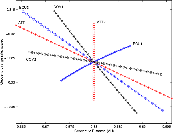	Figure 1: For the asteroid 2004 FU4 the computation of the LOV, by using only the first 17 observations, in different coordinates without scaling. The Cartesian and Attributable LOVs are indistinguishable on this plot and so only the Attributable LOV is depicted.
Open with DEXTER

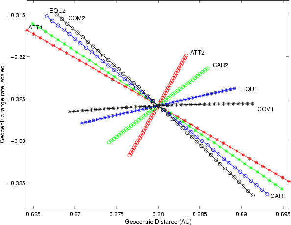	Figure 2: As in the previous figure, but with the scaling of Table 1
Open with DEXTER

Figures 1 and 2 show a comparison of the LOVs computed with different coordinate systems, without and with the scaling defined in Table 1, in the case of asteroid 2004 FU₄ observed only over a time span of $\simeq$3days, with an arc of only $\simeq$$1^\circ$. The data are projected on the $(r, \dot r)$ plane, with $\dot r$ scaled by $n_\oplus$. For each coordinate system we show both the LOV, sampled with 41 VAs in the interval $-1\leq \sigma_Q \leq 1$, and the second LOV, defined as the LOV but with the second largest eigenvalue $\lambda_2$ of the normal matrix and the corresponding eigenvector V₂. The dependence of the LOV on the coordinates is very strong in this case. Note that the LOV of the Cartesian and Attributable coordinates is closer to the second LOV, rather than to the first LOV, of the Equinoctial coordinates.

In such cases, with a very short observed arc, the confidence region has a two-dimensional spine, and the selection of a LOV in the corresponding plane is quite arbitrary. For example, in scaled Cartesian coordinates, the ratio of the two largest semiaxes of the confidence ellipsoid is 2.4. Then the best strategy to sample the confidence region would be either to use a number of LOVs, like in the figures, or to use a fully two-dimensional sampling, as in (Milani et al. 2004a).

Note that the Attributable and the Cartesian coordinates in the unscaled case give almost identical first and second LOV (see Figs. 1 and 3). This can be understood knowing that the $(r, \dot r)$ plane of the Attributable coordinates corresponds exactly to a plane in Cartesian coordinates and, without scaling, the metric on this plane is the same.

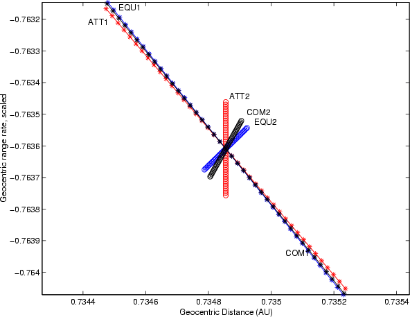	Figure 3: For the asteroid 2002 NT7 the computation of the LOV, by using only the first 113 observations, in different coordinates without scaling. The Cartesian and Attributable LOVs are indistinguishable.
Open with DEXTER

	Figure 4: As in the previous figure, but with the scaling of Table 1.
Open with DEXTER

Figures 3 and 4 show the comparison of the LOVs in the case of asteroid 2002 NT₇ when the available observations were spanning 15 days, forming an arc almost $9^\circ$wide. In this case the ratio of the two largest semiaxes (in scaled Cartesian) is 7.3 and the LOVs computed with different coordinates are very close. As the confidence region becomes smaller, but also narrower, the long axis becomes less dependent upon the metric.

   
3 Application 1: Impact monitoring

The sampling along the LOV is an essential tool whenever the predictions are extremely nonlinear. This happens when the confidence region is very large, at least in one direction, either at the initial epoch (because of very limited observational data) or at some subsequent time (when the propagation is especially chaotic, as in the case of repeated close encounters).

A critical application of confidence region sampling is the so called impact monitoring. For an asteroid with an orbit still largely uncertain we need to know if there is a non-vanishing, although small, probability of collision with the Earth in the next, say, 100 years. Although Monte Carlo sampling with randomly selected VAs is possible, for large asteroids we are interested in detecting very small probabilities of impact (10^-8, even 10^-9) and random sampling would not be efficient enough (Milani et al. 2002).

The use of the LOV in impact monitoring was introduced in (Milani et al. 1999) to sample in a more efficient way the confidence region with VAs more representative of the possible sequence of future close approaches. Milani et al. (2004b) improved the procedure by exploiting the geometrical understanding of the behavior of the LOV as a continuous string.

The computational realization of the structure of the LOV as a differentiable curve is obtained by a version of the same method described in Sect. 2.5. Given two VAs with consecutive index, X_k and X_k+1, corresponding to the values $\sigma_k$ and $\sigma_{k+1}$ of the parameter, VAs with non-integer index corresponding to values $\sigma_k<\sigma<\sigma_{k+1}$ can be obtained by first performing an approximate integration step

$$X'(\sigma)=X_k+(\sigma-\sigma_k)\;F(X)$$

and then constrained differential corrections until convergence to the LOV point $X(\sigma)$.

In this application, when the impact is not immediate but results from a resonant return, what matters most is sampling with VAs the values of the semimajor axis compatible with the available observations. In such cases the choice of coordinates and scaling is not critical. As an example, Figs. 3 and 4 refer to a case relevant for impact monitoring: with the 113 observations available until July 24, 2002, there was a probability of 1/90 000for an impact of 2002 NT₇ on February 1, 2019.

On the contrary, when the observations cover only a short arc and there is a possibility of impact at the first close approach to the Earth, the choice of the coordinates and scaling in the definition of the LOV can make a significant difference in the output of the impact monitoring systems. Figures 1 and 2 refer to the case of 2004 FU₄, for which there was a Virtual Impactor in 2010 with probability $~4\times 10^{-8}$. We tested the CLOMON2 impact monitoring system by using Equinoctial, Cartesian and Attributable elements, with and without scaling, selecting the first and the second LOV. Of these 12 combinations, only 3 allowed to detect the 2010 VI, namely the scaled Equinoctial first LOV and the Cartesian/Attributable scaled second LOV. The same VI was also found by Sentry with scaled Cometary elements (first LOV). Looking at Fig. 2 it is clear that the four LOVs starting from which the 2010 VI was found are close together.

   
4 Application 2: Orbit determination

The procedure based on constrained differential corrections (Sect. 2.4) to obtain LOV solutions can be used starting with an arbitrary initial guess X, which can be provided by some preliminary orbit. It can also be used starting from a known LOV solution (be it the nominal or not) as part of the continuation method (Sect. 2.5) to obtain alternate LOV solutions. In both cases it can provide a richer orbit determination procedure.

   
4.1 LOV solutions from preliminary orbits

We can conceive a new procedure for computing an orbit starting from the astrometric data. It consists of the following steps:

1.

if some orbit X is already available, it is used as preliminary;

2.

if no orbit is available, a preliminary orbit X is computed, e.g., with Gauss' method, but also with other methods suitable for short arcs (Milani et al. 2004a);

3.

if the preliminary orbit algorithm fails, the orbit determination procedure is considered failed;

4.

if the preliminary orbit X is available, constrained differential corrections are computed starting from X as first guess;

5.

if constrained differential corrections converge to a LOV solution $X_{\rm LOV}$ (with rms of the residuals $\leq \Sigma$) then a full differential correction is attempted by using $X_{\rm LOV}$ as first guess;

6.

if the full differential corrections converge to a nominal solution X^* (with rms of the residuals $\leq \Sigma$) then this is adopted as orbit (with uncertainty described by its covariance);

7.

if the full differential corrections fail, then $X_{\rm LOV}$ is adopted (if available, and with rms $\leq \Sigma$) as orbit;

8.

if the constrained differential corrections fail to converge we start differential corrections with the preliminary orbit X as first guess;

9.

if these differential corrections converge to X^* (with rms of the residuals $\leq \Sigma$), it is then adopted as orbit;

10.

if this last attempt fails the orbit determination procedure is considered to be failed.

The logic is also represented in the flowchart (Fig. 5).

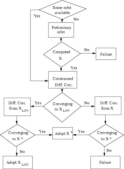	Figure 5: Orbit computation flowchart.
Open with DEXTER

After obtaining a least squares orbit, be it a nominal or just a LOV solution, we can apply the continuation algorithm of Sect. 2.5 for multiple LOV solutions.

By this procedure, it is possible to obtain a significantly larger number of orbits. The increase results from:

• LOV solutions in cases where nominal solutions are not available;
• nominal solutions computed thanks to the intermediary of the LOV orbit, while the iterations starting from the poorer preliminary orbit would diverge;
• multiple LOV solutions computed by continuation from all the available nominal solutions;
• multiple LOV solutions computed by continuation from all the LOV solutions obtained directly from the preliminary orbit, when no nominal is available.

A quantitative assessment of this increase in the orbit catalogs is obtained from the large scale test of the following section.

4.2 Large scale orbit determination test

The results of a large scale application of the procedure described above to compute as many least squares orbits as possible, and then to explicitly sample the LOV with VAs, are as follows.

We have used all the astrometric data on unnumbered asteroids as made public by the Minor Planet Center on the 9th of November, 2003 (7.5million observations). We have computed as many least squares orbits as possible among the 233 411 designations corresponding to independent asteroid discoveries.

The procedure described above was applied to all designations, in Equinoctial coordinates (unscaled) and with the control value for the normalized rms of the residuals set to $\Sigma=3$. Note that in this test the modern (after 1950) observations have been weighed at 1arcsec, thus normalized ${\rm rms}=3$ essentially means unnormalized ${\rm rms}=3$ arcsec. If more than one preliminary orbit is available, e.g., from the existing catalogs, from Gauss' and from other preliminary orbit methods, in case of failure we repeat the procedure starting from each preliminary orbit. The final outcome can thus be either a full orbit, or a constrained orbit, or a complete failure.

The relative number of successes in the orbit determination procedure depends upon the quality of the data for the designations. For this purpose, we classify the designations in 7 quality classes by the length of the observed arc, the number of observations and the number of nights in which they have been taken, as described in Table 2.

Table 2: Classification of the designated asteroids according to the amount and timing of the available astrometry.

Clearly, the data of the best qualities are such that in almost all cases either a nominal, or at least a LOV solution can be computed; as the quality decreases the relative number of orbit-less designations increases. As an example, for the 78 672 quality 1 cases a nominal orbit has been computed (by converging full differential corrections) in all cases. For these orbits, essentially coinciding with the multi-opposition asteroids, the uncertainty (as measured by the linear confidence region $Z_{\rm L}(3)$) is so small that the usage of LOV methods for future prediction is generally not necessary. However, there are exceptions: by consulting the AstDyS online service providing ephemerides with sky plane uncertainties for all the multi-opposition asteroids, we can find 14 cases with a sky-plane uncertainty ellipse with a major axis exceeding $6^\circ$ and another 23 exceeding $3^\circ$. To recover these, the LOV methods can be very useful.

For qualities 2, 3 and 4, that is for asteroids observed at a single apparition but in at least three separate nights, almost all, actually $99.7\%$ of the objects, ended up with a full least squares orbit (see Table 3).

For qualities 5 and 6 (two-nighters) a significant fraction of the output orbits was constrained, that is, a constrained orbit was computed, but the attempt to use it as first guess for a full differential correction failed. Moreover, of the nominal solutions computed, a significant fraction was obtained only by using a LOV solution as intermediary. For a two-nighter, Gauss' method for preliminary orbit is unreliable, and the full differential corrections starting from it often diverge.

Table 3: The performance of the various preliminary orbit determination strategies discussed in the text.

For quality 7 (one-nighters) the number of full least squares orbits is very small, even the constrained orbits are few ($3\%$), moreover the uncertainty of these orbits is quite ridiculous.

The comparison with the classical differential correction algorithm, without passing through the constrained computations (Col. "D. C.'' in Table 3) shows that a large number of complete orbits have been computed only by means of the intermediate step provided by the constrained solutions. The number of such cases is not large (a few hundreds) for objects observed in at least 3 nights (quality 2-4), but there are thousands of new orbits obtained in this way for two-nighters (quality 5 and especially quality 6).

In the discussion of identifications, in the following section, both the orbits remaining as constrained and the complete ones obtained passing through the constrained contribute to the catalogs of orbits, and therefore to the increase on the number of possible identifications. The question, of course, is whether these additional orbits are good enough to be useful, and this is discussed in Sect. 5.

For all the cases of quality 2 to 7 in which we have been able to compute a least squares orbit (be it full or constrained), we have applied the multiple solution computation by continuation of Sect. 2.5 (again in unscaled Equinoctial elements), attempting to compute 21 VAs (including the one used as starting point, that is 20 additional solutions) for each designation. The results are shown in the last column of Table 3 and, as expected, are very good for qualities 2, 3 and 4, that is almost all the sought for VAs have been computed.

For quality 5 and 6 the results are good, but their interpretation is less straightforward, because many multiple solutions have been computed starting from constrained solutions. The multiple solutions obtained in this case can still be considered as VAs, sampling the LOV but not "centered'' in the segment of the LOV corresponding to lower values of the residuals normalized rms. On the other hand, the two-nighters are the objects for which the observational information is not enough. Even when a nominal orbit can be found, it typically has an enormous uncertainty: ${\rm rms}(a)> 1$ AU is common, and ${\rm rms}(e)> 1$does occur, that is, a large fraction of the nominal orbits are not significantly better than a constrained orbit. Then these are the objects for which recovery or identification is absolutely necessary, thus they are the ones on which testing innovative algorithms is more important.

   
5 Application 3: Orbit identification

The designations correspond to independent asteroid discoveries, but they do not necessarily correspond to physically different objects. Identification is the process by which two (or more) designations are found to contain observations of the same object, by computing a least squares fit to all the observations, with acceptable residuals. The difficulty is not as much in testing one identification once it has been proposed: this is done by using differential corrections and outlier rejection (Carpino et al. 2003). Rather, the problem is how to decide among the $\simeq$ $230~000\times 230~000/2$ couples which ones should be tested as candidates for identification. Of course this requires some filtering procedure, selecting couples of designations on the basis of some metric describing similarity between the two.

The procedures to propose identifications belong to different types, essentially depending upon the quality of observational data available for each designation. We use the classification given in (Milani 1999), and in this paper we shall discuss mainly orbit identifications and briefly attributions (in the last Subsection). We only marginally discuss linkages, which will be the subject of further research. The procedure for recovery of a lost asteroid (by finding it either in the sky or in the image archives) using the multiple solutions method has been thoroughly discussed in (Boattini et al. 2001).

   
5.1 The orbit identification algorithm

Orbit identification applies to the case where both designations have a least squares orbit (which could be a nominal solution, but also a constrained solution). The procedure involves the computation of a sequence of similarity metrics between the nominal solutions of some pair of designations, taking also into account their uncertainty (as expressed by the covariance matrix). The method is described in (Milani et al. 2000) and we will only briefly summarize it here.

Let X₁ and X₂ be the least squares solutions (at the same epoch) for the two designations and let C₁, C₂ be the corresponding normal matrices. The two cost functions of the two separate orbit determination processes are:

$$\begin{eqnarray*}Q_i(X)&=&Q_i(X_i)+ \frac 1{m_i}~ (X-X_i)\cdot C_i~(X-X_i) + \ldots\\ &=& Q_i^* + \Delta Q_i ;\quad i=1,2 , \end{eqnarray*}$$

where m_i is the number of scalar residuals.

For the two orbits to represent the same object we need to find a low enough minimum for the joint cost function, formed with the sum of squares of the m=m₁+m₂ residuals:

$$\begin{eqnarray*}Q&=& \frac 1m (m_1Q_1 + m_2 Q_2)\\ &=& \frac 1m ~ ( m_1 Q_1^*+ ... ...1 + m_2 \Delta Q_2)\\ &=& Q^* + \Delta Q = Q^*+ \frac{\chi^2}m \end{eqnarray*}$$

where Q^* is the value corresponding to the sum (with suitable weighting) of the two separate minima.

The linear algorithm to solve the problem is obtained when the $\chi^2$ value is approximated by the sum of the quadratic approximations of the separate $\Delta Q_i$:

$$\chi^2\simeq (X-X_1)\cdot C_1~(X-X_1) + (X-X_2)\cdot C_2~(X-X_2).$$

The minimum for $\chi^2$ can be found by minimizing the non-homogeneous quadratic form above. If the new joint minimum is X₀, then by expanding around X₀ we have

$$\chi^2 \simeq (X-X_0)\cdot C_0~ (X-X_0) + K$$

and by comparing the last two formulas we find:

$$\begin{eqnarray*}C_0&=&C_1+C_2\\ X_0&=&C_0^{-1}~ (C_1~ X_1 + C_2~ X_2)\\ K&=& X_1\cdot C_1~X_1 + X_2\cdot C_2~X_2 -X_0\cdot C_0~ X_0 \end{eqnarray*}$$

providing the new minimum point. The expected $\chi^2$ value K for the identification, corresponding to X₀ (in the linear approximation), is given by another quadratic form

$$K= \Delta X \cdot C~ \Delta X$$

where $\Delta X=X_2-X_1$ is the difference of the two orbital element sets, and the symmetric matrix C is given by

C= C₁-C₁  C₀^-1  C₁= C₂-C₂  C₀^-1  C₂ .

The orbit identification penalty K is computed and used as a control to filter out the couples of orbits which cannot belong to the same object (unless the observations are exceptionally poor). To the orbit couples passing this filter we apply the differential correction algorithm, with X₀ as first guess.

This algorithm has been used successfully, but it is far from detecting all the identifications which are hidden in the data. The main limitation is typical of the algorithms based upon linearization: if the difference $\Delta X$ is not small, assuming that the normal matrices C₁, C₂ (and consequently C₀, C) are independent from the point X where they are computed is a poor approximation.

Our new algorithm strives to decrease the size of the penalty K for candidate couples for identification, thus revealing them as a priori more suitable for identification. This is obtained by replacing the nominal solutions X₁, X₂ with two sets of VAs X₁⁽ⁱ⁾, X₂^(k), with i,k=1,N_m (in the tests of this paper, $N_m\leq 21$, as described in Table 3). Then we compute K_i,k, the expected value of $\chi^2$ for the identification between each pair of VAs, and select the two indexes i,k corresponding to the minimum value $K_{\rm min}$. If this minimum is low enough, the pair of designations is proposed for identification, using as first guess the value X₀ as computed for these two VAs.

   
5.2 Comparative tests

The main goal of this paper is to show the advantages of the new algorithms with respect to the previous ones. Thus we need to measure how many reliable identifications can be found with the new methods, on top of the ones found by a thorough application of some previous method. For this purpose, we have performed three full computations on exactly the same observational data for unnumbered (but designated) asteroids made public by the MPC in November 2003:

Nominal Single (NS) solution:

we have applied the orbit identification algorithm (Milani et al. 2000) to a catalog of nominal orbits obtained through the classical method of differential corrections.

Constrained Single (CS) solution:

we have computed the orbits by exploiting the use of the constrained differential correction as first step, as described in Sect. 4, and then we have searched for the orbit identifications with the same algorithm as in (Milani et al. 2000), but using the enlarged set of orbits.

Constrained Multiple (CM) solutions:

we have used the same extended set of orbits, but tested the multiple solutions identification algorithm described above.

For the sake of simplicity, when referring either to these three tests or to the corresponding algorithms, hereafter we will denote them by "NS'', "CS'' and "CM'' respectively, although we will mainly focus on the comparison between the last two.

Analysis of the outputs

The overall numbers associated with the different tests are summarized in Table 4. The main conclusion is the superiority of the algorithm based on multiple solutions: the number of proposed identifications is more than three times the number obtained by the CS method and more than ten times the amount got in the NS test. Besides, out of the 11 737 proposed identifications only 7.6% were not included among those found by the CM method and only 0.6% were not found by at least one of the two methods CS and CM.

Table 4: Summary of the tests' results.

A breakdown of the results obtained in the tests is displayed in Table 5, which shows the number of identifications that have been proposed by the CS and the CM algorithms (first row), as well as the subset of identifications that could not be found in the NS test (second row). The role played by the constrained orbits becomes apparent from the data included in the third and fourth rows: 55% of the identifications found only by the CS and CM methods involve at least one asteroid with constrained orbit. This feature is even more remarkable when the attention is restricted to those identifications only proposed by the CS method, where the percentage raises to 82%.

Table 5: A detailed analysis of the identifications proposed by the CS and CM methods.

Table 6: As in Table 5, but for published identifications.

Clearly, a first indication of the power of any of the algorithms is given by the number of proposed identifications (the more the better!). However their final reliability will be measured by counting the fraction of proposed identifications that reach publication: this implies the residuals of the proposed identifications have been inspected (first by us, then by the MPC) and found to be indicative of a good fit, without suspicious trends and systematic effects. The third row in Table 4 summarizes the number of identifications that have been published for each algorithm. Table 6 gives the same data as in Table 5 for the identifications which have been published.

Once again, the CM method provides the most remarkable results. Moreover, the comparison between the results obtained by the CS and CM procedures shows that only a very small percentage ($\sim$$2.75\%$) of published identifications found by the former escape to the latter.

Particularly interesting are those identifications in which the two asteroids involved have a constrained orbit. Among them, the most outstanding cases are those in which the proposed identification has been confirmed by an additional identification with a third asteroid. Examples of such a situation are:

$$\begin{array}{lllll} \mbox{1992 SB}_3 & = & \mbox{2000 PG}_{1... ...& = & \mbox{1996 VJ}_{21} & = & \mbox{2000 TU}_{71} \end{array}$$

where the last two identifications were obtained in both the CS and CM tests, whereas the first three were only found by the CM method. Also remarkable in these examples is the fact that, except for the last case, the first two asteroids of each identification were two-nighters.

The superiority of the CM method is clear from the data analysis presented so far. This conclusion is reinforced when we take into account that the tests have been performed six months after the observational data set was issued. The critical test is then to measure how many of the published identifications are credited to our group by the MPC. This means that the identification is not only reliable, but has not been found before by other groups, even though they had all the time to try. In fact, as shown in the last row of Table 6, over 50% of the published identifications are credited to us.

Working with a comparatively old data set has the advantage that most of the published identifications are well established, allowing more reliable conclusions on the efficiency of the algorithm, moreover all the new identifications found are a confirmation that our new methods reach farther than the previously known methods of identifications.

With the NS method, which has been in use since 1999, to have a good fraction of the identifications credited to us required to process the data in a very short time, as soon as the data were available. With the new CS and CM methods, more than 52% of the identifications credited to us involve two objects discovered before January 1, 2003. This percentage reaches 91% for a discovery date before October 1, 2003 (one month before the observational data set used in this paper was issued). There is no need to rush to get the results before the competition.

Improving the filter parameters

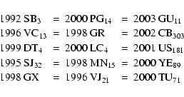
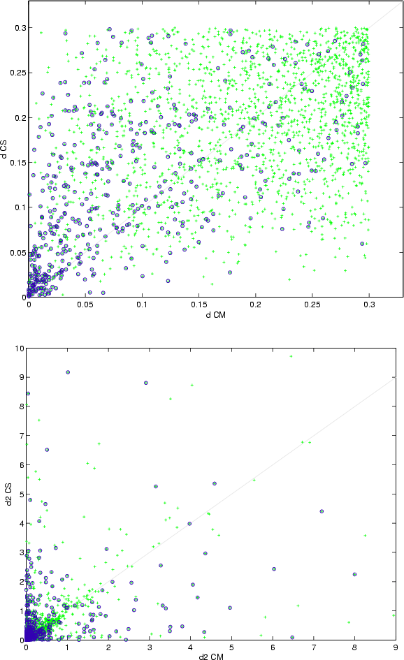Figure 6: Comparison of the filter values d ( up) and d2 ( bottom) for the identifications simultaneously obtained in the CS and CM tests. Each plot shows, using crosses, the values taken by a filter parameter in both methods. The crosses marked with a circle correspond to published identifications. The straight line marks the location where the values of the metrics is equal for both methods (those points above this line represent identifications in which the multiple-solutions algorithm improves the value obtained by the single-solution method).

Open with DEXTER

	Figure 7: As in Fig. 6, but for distances d5 and d6.
Open with DEXTER

The practical implementation of the tested algorithms are based on the computation of a number of semi-norms, introduced in (Milani et al. 2000), each one computed as the square root of an identification penalty in some subspace. The most simple, called d, is exclusively based on the difference of the Equinoctial orbital elements:

$$\small d= \sqrt{\left(\frac{a_1-a_2}{a_1+a_2}\right)^2 + (h_1-h_2)^2 + (k_1-k_2)^2 + (p_1-p_2)^2 + (q_1-q_2)^2} .$$

In addition, we use the following three metrics that depend not only upon the orbital elements but also upon the uncertainties:

• d₂ is based on the equinoctial elements p and q whose definition include the orbital inclination, a quantity usually well determined from the observational data;
• d₅ uses five orbital elements, leaving out the mean longitude that usually carries the biggest uncertainty (and is responsible for most of the nonlinearity);
• d₆, uses the full set of equinoctial elements; note that, for the same couple of orbits, $d_6\geq d_5$ (Milani et al. 2000, Sect. 2.3).

Those metrics, initially designed to handle nominal solutions, have been suitably adapted to the multiple-solution context.

The first stage in the orbit identification algorithms is to apply these metrics as a cascading series of filters on each pair of asteroids. For each distance metric we select a limit value, beyond which the distance is deemed too great to deserve further testing. The metric filters are sequentially applied in the order above: this corresponds to an ascending order in accuracy and computational complexity. The increase in computational load is balanced by the decreasing number of pairs that reach each successive filter. Those pairs that successfully pass all the filters in the first stage (the proposed pairs of Table 4) are sent to a least squares fit and are recognized as proposed identifications when the corresponding differential correction algorithm is convergent to an orbit with an acceptable rms.

Another motivation for the comparative tests between the CS and CM algorithms was to investigate the behavior of the different filters, with the goal of fine tuning the cutting values for efficiency and reliability of the detection of identifications.

The plots in Figs. 6 and 7 provide a direct comparison of the filter values for those identifications simultaneously obtained by the CS and the CM methods. The interpretation is as follows: points with a better filter value in the CM than in the CS method are located above the diagonal lines. The main feature shown in those pictures is the migration of the cloud of points to the upper half as the quality of the filter increases. This means that, as expected, in most of the cases the CM algorithm significantly lowers the identification penalty between orbits and, hence, the nonlinearity of the problem. Note that this is exactly the goal we were pursuing when introducing the multiple identification algorithm at the end of the previous subsection.

For each filter, Table 7 shows the precise percentage of proposed identifications that improve the metric value in the CM test with respect to that obtained by the CS one. The percentage of improved values barely exceeds 50% for the first filter and it almost reaches 100% for the last filter. When the analysis is restricted to the published identifications, the corresponding percentages are larger.

The histograms collected in Fig. 8 refer not only to the common identifications found by the CM and the CS tests but to the whole population of proposed (void bars) and published (solid bars) identifications found by each method. These histograms depict the normalized distribution of the values for the different filters used.

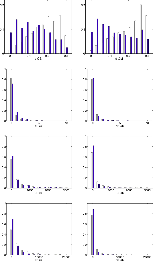	Figure 8: Normalized histograms for the values of the four filter distances (CS, left and CM, right). Each figure showsthe relative distribution of values of a given filter: void bars for all proposed identifications, solid bars for the published ones.
Open with DEXTER

Table 7: CM vs. CS: improvement of the metric values.

Another comparison of the different metrics is given in Table 8, which shows several percentiles for the distribution of values of each distance. Even though the results displayed for the d distance are slightly worse for the CM algorithm, its superiority is rather evident for the other metrics. For instance, to find 95% of the published identifications, the CM method lowers by a factor 2 the percentile values of d₅ and d₆ with respect to those needed by CS.

Table 8: Some percentiles for the distributions of the filter values as obtained for the published identifications found in the CS and CM tests.

To understand these results, we need to take into account two competing effects. On one hand, the CM method decreases all the distances by selecting the minimum among a finite set of couples of VAs. On the other hand, the size of the catalog of orbital elements used as input to the identification filters is so huge in the CM method that it is difficult to handle. Thus we have given up, in the CM method, one device used in the NS and CS methods: given one input catalog of orbits, we propagate it to a number of different epochs (e.g., 5 epochs in this test). For each couple of designations being tested, we select the catalog with epoch closest to the midpoint of the two discovery dates (Milani et al. 2000, Sect. 5). Thus in the CM method the covariance of the orbital elements is, in most cases, propagated for a longer time span: this increases the size of the confidence region and enhances the nonlinear effects.

Thus the data shown in the figures and tables of this subsection indicate that the CM method is not effective in decreasing (with respect to the CS method) the value of the d distance, and only marginally effective in decreasing d₂. The advantage of the multiple solutions method becomes very significant for the d₅ and d₆ metrics, apparently by far exceeding the negative effect of the lack of the multiple epochs catalogs.

Finally, we have used the extensive tests to perform a fine tuning on the selection of the cutting values for the different filters in order to maximize the results with minimum computational effort.

A good measure of the performance of each algorithm is provided by the ratio between the number of published and proposed identifications. Since testing proposed identifications by differential corrections is the most computationally intensive step of the procedure, this corresponds to the results over cost ratio. Therefore, we aim at selecting the filter cutting values in such a way that this ratio is maximum.

Table 9: Filter cutting values: optimal selection.

To achieve this goal we have used a discrete four dimensional grid that results from taking equally spaced nodes in the range of variation of each of the four distances. In this grid we have selected those points for which a fixed percentage of published identifications are lost. The optimal choice for the filter cutting values corresponds to the point of the grid that makes maximum the number of discarded potential identifications (i.e., maximizes the ratio between published and proposed identifications). The results of this computation, for several percentages of published identifications that we would be accepting to lose, are given in Table 9.

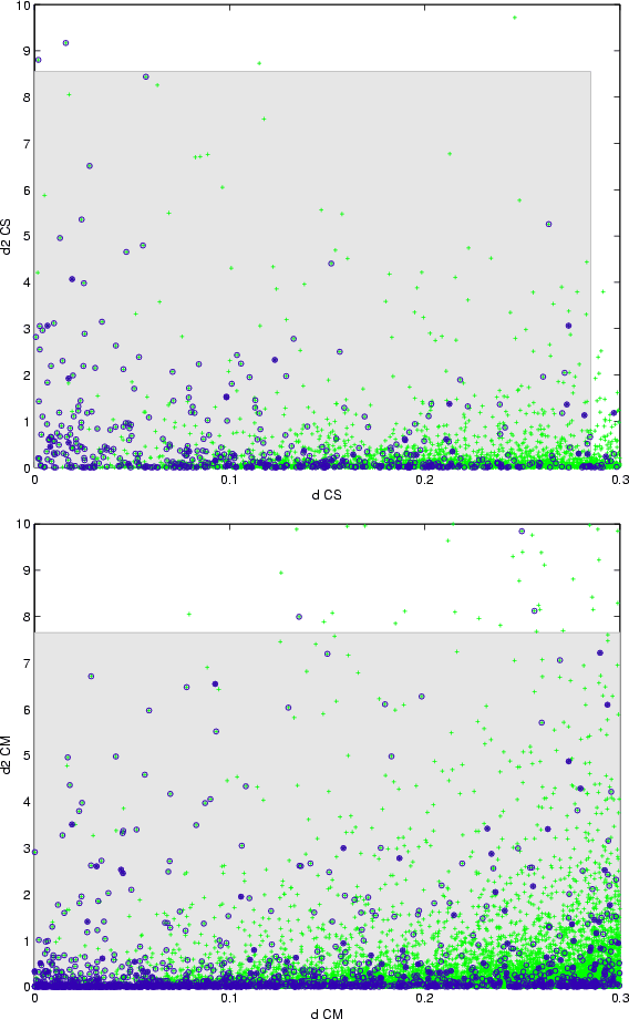	Figure 9: Distribution of identifications obtained by the CS ( up) and CM ( bottom) methods in the d-d2 plane. Each proposed identification is represented by a single cross. Encircled crosses correspond to those published. Shaded rectangles are optimal regions (at the 5% loss level).
Open with DEXTER

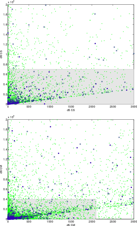	Figure 10: As in Fig. 9, but in the d5-d6 plane. Note that in exact arithmetic $d_5\leq d_6$. The exceptions (below the diagonal in the plots) indicate numerically unstable cases, with very badly conditioned normal matrices. These extremely unstable computations nonetheless provide some reliable identifications!
Open with DEXTER

Except for the lower percentages, where the cutting values tend to equalize in both methods, we observe again slightly greater values for d in the CM method and substantial lesser values for the other metrics, which is consistent with the comments made above on the behavior of the distributions. This situation is displayed in the plots collected in Figs. 9 and 10, which show the optimal parameter region for both algorithms when the maximum percentage of lost published identifications is fixed at 5%.

In summary, from the massive tests carried out, we can conclude that the algorithm based in the computation of multiple solutions for each asteroid represents a great advance towards the solution of the asteroid identification problem: it allows us not only to find many more identifications, but also those which are more difficult and have been hidden in the catalogs for a long time. Nevertheless, there is room for improvement at least in two areas. First, we would like to improve efficiency, since not all the steps of the procedure have yet been optimized: e.g., the very time consuming check of the residuals to decide which proposed identifications are worth submitting for publication requires much more automation. Second, we can aim at a more complete search for identifications, possibly exploiting the freedom to choose coordinates, scaling and the second eigenvalue in the definition of the LOV. The current test has been conducted using the Equinoctial coordinates, no scaling and the first LOV; as it is clear from Sect. 2.6, different proposed identifications could easily be obtained with other choices.

   
5.3 Observation attribution

We now discuss attributions of a set of observations, for which a set of orbital elements is not available, to another discovery for which there are enough observations to compute a least squares orbit. We shall not repeat the formulas of the linear attribution algorithms (Milani et al. 2001) because they are conceptually the same as those shown in Sect. 5.1, with a different interpretation for the symbols.

Let X₁ be an attributable, that is a 4-dimensional vector representing the set of observations to be attributed; its coordinates are $(\alpha, \delta, \dot \alpha, \dot \delta)$, that is the same as the first four components of an Attributable elements set. To compress the information of a set of observation, forming a small arc on the celestial sphere, into representative angles and angular velocities, we use a fit to a low degree polynomial of time, separately for $\delta$ and $\alpha$. Let C₁ be the normal matrix of such a fit.

Let X₂ be a predicted attributable, computed from a known least squares orbit. Let $\Gamma_2$ be the covariance matrix of such an attribution, obtained by propagation of the covariance of the orbital elements (as obtained in the least squares fit, be it full or constrained). Then $C_2=\Gamma_2^{-1}$ is the corresponding marginal normal matrix.

With this new interpretation for the symbols X₁, X₂, C₁, C₂, the algorithm for linear attribution uses the same formulas of Sect. 5.1, with the identification done in the 4-dimensional attributable space. In particular, the attribution penalty K is computed and used as a control to filter out the pairs orbit-attributable which cannot belong to the same object (unless the observations are exceptionally poor). To the pairs orbit-attributable passing this filter we apply the differential correction algorithm, with the known orbit as first guess.

This algorithm is effective whenever the distance (in the 4-dimensional attributable space) between X₁ and X₂ is not too large and the penalty is small, thus the linear approximation is accurate. Let us suppose this is not the case because the prediction X₂ has a large uncertainty (i.e., $\Gamma_2$ has large eigenvalues); this can be due either to a weak orbit determination at the epoch of the observations, or to a long propagation, because the two designations have been discovered far in time from each other. Then the confidence region of the prediction X₂ is not well represented by the confidence ellipsoid

$$Z_{\rm L}(X_2)=\left\{X \vert (X-X_2)^T\; C_2\; (X-X_2)\leq \chi^2 \right\} .$$

In this case it is appropriate to sample in a nonlinear way the confidence region in the attributable space by using the LOV. This leads to a new algorithm, in which the attribution penalty K_i is computed for each of the VAs (indexed by the integer i) computed along the LOV. If at least some of the K_i are low, then X₁ may be attributed to the orbit giving the prediction X₂.

This algorithm is more effective than using the nominal prediction only, and indeed it has been used to generate new attributions on top of the ones already obtained with the single orbit method. However, unlike the case of the orbit identifications, it is not easy to assess how significant is the improvement. This for two reasons. First, we have obtained such an improvement in the orbit identification procedure by using multiple solutions that, after running the large scale test of Sect. 5.2, a large fraction of the attributables correspond to designations with some least squares orbits (including the constrained ones) and most identifications have already been obtained. Therefore, it is difficult to separately measure the improvement in the attribution algorithm. Second, the attributions are often questionable when the attributable is computed only over a short observations time span. Hence, to confirm them it is essential to be able to find a third discovery corresponding to the same object. The possibility of doing this is critically dependent on the availability of enough short arc data. Thus we plan to perform a more specific large scale test of the attribution to multiple solutions by processing a much larger database of independent short arc discoveries.

   
6 Application 4: Qualitative analysis

The sampling along the LOV is also useful to understand the situation whenever the orbit determination is extremely nonlinear.

The problem of nonlinearity in orbit determination is too complex to be discussed in full generality here. We would like to show the use of the LOV sampling as a tool to understand the geometry of the nonlinear confidence region in a single, difficult example, in which there are multiple local minima of the cost function.

The asteroid 1998 XB was discovered on December 1, 1998, while it was at an elongation of $\simeq$$93^\circ$ from the Sun. The first orbit published by the MPC, based on observations over a time span of 10 days, had a semimajor axis a=1.021 AU (MPC 1998). In the following days the orbit was repeatedly revised by the MPC, with semimajor axis gradually decreasing until 0.989 when the observation time span was 13 days. Then, with the addition of observations extending the time span to 16 days, the semimajor axis jumped to 0.906.

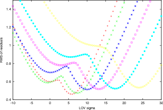	Figure 11: The rms of the residuals (in arcsec), as a function of the LOV parameter $\sigma$, for different amounts of observational data. The lines are marked with plusses (arc time span of 9 days), crosses (10 days), stars (11 days), boxes (13 days), full boxes (14 days) and circles (16 days)
Open with DEXTER

To understand the bizarre behavior of this orbit determination we can compute the LOV for different data, corresponding to observed time spans of 9, 10, 11, 13, 14 and 16 days. As Fig. 11 shows, the rms of the residuals along the LOV has a double minimum: the secondary minimum moves, as the data increase, in direction of lower a, but not as far as the location of the other minimum. The secondary disappears only with 16 days of data, and then the differential corrections lead to the other solution.

It is well known (Marsden 1985) that Gauss' method for determining an orbit from three observations can have two distinct solutions when the elongation is below $120^\circ$. When applied with three observations selected in the shorter time spans, it can provide preliminary orbits close to both the primary and the secondary minimum.

As an example, with data over 10 days we can compute a preliminary orbit by Väisälä's version of Gauss method, with a=0.900, and from this a full least squares solution with a=0.901 and rms 0.47arcsec. If we use the Merton version of Gauss' method we get a preliminary solution with a=1.046, and from this we can compute a "nominal'' solution, that is a local minimum, with a=1.032 and rms 0.58 arcsec.

This example confirms that the region with elongation around $90^\circ$ is especially difficult for orbit determination, but also shows that the LOV can provide a very efficient tool to understand complex nonlinearities.

7 Conclusions

In this paper we have introduced a new definition of Line Of Variations, rigorously applicable in all cases (including the strongly perturbed orbits) and explicitly computable thanks to the algorithm of constrained differential corrections and to the continuation method.

This definition depends upon the metric, thus upon the coordinates and scaling used. In practice the different LOVs give the same results when enough observations are available. For objects observed only over a very short arc, the LOV is strongly dependent upon the metric. When the confidence region is essentially flat, two dimensional, the LOV cannot be fully representative. This occurs for most objects observed only over a single night; for two-nighters, sampling of the confidence region by using the LOV is effective for some applications (such as orbit determination and identification) but can be problematic for others (such as impact monitoring).

The concept of LOV and the algorithms to compute it have several applications.

1.

Impact monitoring: it is now possible for near Earth asteroids observed for only a few days, although this may not be enough to detect possible impacts after just one night of observations.

2.

Orbit determination: by using LOV solutions as intermediary, and also as replacement of the nominal solution, we have obtained a huge increase of the size of asteroid orbit catalogs.

3.

Orbit identification: two effects, larger input catalogs and the use of multiple LOV solutions to mitigate nonlinearity, together account for an increase in the number of identifications by an order of magnitude.

4.

The LOV is a useful tool for qualitative analysis of difficult cases with extreme nonlinearity.

Acknowledgements

This research has been supported by the Spanish Ministerio de Ciencia y Tecnología and by the European funds FEDER through the grant AYA2001-1784. This research was conducted, in part, at the Jet Propulsion Laboratory, California Institute of Technology, under a contract with the National Aeronautics and Space Administration.

   
Appendix A: Comparison of LOV definitions

To obtain rigorous results, we need to use also the weak direction vector field for Newton's method

$$C^N(X)~V^N_1(X)= \lambda^N_1(X)\;V^N_1(X)$$

with |V^N₁|=1, $\lambda^N_1$ the lowest eigenvalue.

$$F^N(X)= \pm \frac{1}{\sqrt{\lambda^N_1(X)}}\; V^N_1(X).$$

Definition LOV1. The solution of the differential equation

$$\frac{{\rm d}X}{{\rm d}\sigma}= F(X)$$ (A.1)

with initial conditions X(0)=X^* (a nominal solution).

Definition LOV2. The solution of the differential equation

$$\frac{{\rm d}X}{\rm d\sigma}= F^N(X)$$ (A.2)

with initial conditions X(0)=X^*.

Definition LOV3. The set of points X such that

 

V₁(X) || D . (A.3)

Definition LOV4. The set of points X such that

 

V^N₁(X) || D . (A.4)

Definition. A solution of the differential equation

$$\frac{{\rm d}X}{\rm d\sigma}= k(X) D(X) ,$$ (A.5)

with k(X) a (positive) scalar function, is called a curve of steepest descent. Such curves have as limit for $s\to+\infty$ a nominal solution X^* (almost always; exceptional curves can have a saddle as limit).

LOV1 and LOV2 are not the same curve. The two curves are close near X^* (provided the residuals are small), they become very different for large residuals and especially near a saddle. LOV3 and LOV4 are not the same curve.

LOV3 and LOV4 do not imply that the curve contains a nominal solution; indeed a minimum may not exist (it may be beyond some singularity, such as e=1 if the elements are Keplerian/Equinoctial). However, if these curves pass in the neighborhood of a minimum, then they must pass through it.

In a linear case $\Xi=B(X-X^*)+\Xi^*$, with B constant, all the definitions LOV1-LOV2-LOV3-LOV4 are the same (and they all are curves of steepest descent).

Theorem: if a curve satisfies LOV4 and either LOV2 or it is of steepest descent, then it is a straight line.

Proof. If LOV4, then there is a scalar function h(X) such that F^N(X)=h(X) D, thus LOV2 and being of steepest descent are equivalent. Let us select the particular steepest descent curve

$$\frac{{\rm d}X}{{\rm d}\sigma}= D$$

and let us reparameterize the curve by arclength s, with

$$\left \vert\frac{{\rm d}X}{{\rm d}s}\right\vert=1 \Longleftrightarrow \frac{{\rm d}s}{{\rm d}\sigma}=\vert D\vert$$

then

$$\frac{{\rm d}X}{{\rm d}s}= \hat D$$

the unit vector in the direction defined by D. Taking into account that

$$\frac{\partial D}{\partial X} = - C^N ;\quad \frac{{\rm d}D}{... ... D}{\partial X} \; \frac{{\rm d}X}{{\rm d}s} = - C^N ~\hat D ,$$

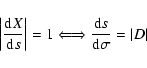
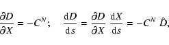
let us compute

$$\frac{{\rm d}^2X}{{\rm d}s^2} \frac{{\rm d} }{{\rm d}s}~ \frac{D}{\vert D\vert}= \frac 1{\vert ... ...ac {\left\langle D, \frac{{\rm d}D}{{\rm d}s} \right \rangle}{\vert D\vert^3}~D$$ =

$$\frac{-1}{\vert D\vert}\; \left[C^N~\hat D - \left\langle\hat D, C^N~ \hat D\right\rangle\hat D\right]$$ =

and if we use LOV2 (or even a weaker condition that D is parallel to some eigenvector of C^N)

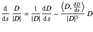$$C^N \hat D = \lambda \hat D \Rightarrow \frac{{\rm d}^2X}{{\r... ...t D, \lambda \hat D\right\rangle~ \hat D\right] = \underline 0$$

thus the curve must be a straight line.

In conclusion we have adopted LOV3 as definition of the LOV, because it is the one actually computable with standard tools, without computing the second derivatives of the residuals and without incurring in the numerical instabilities found in computing LOV1-LOV2. Definitions LOV2 and LOV4 are not equivalent, and they are indeed different curves apart from very special cases, where they are straight lines. We have not been able to prove that definitions LOV3 and LOV1 give different curves, but given the proven result LOV2 $\neq$ LOV4 we expect that also LOV1 $\neq$ LOV3 apart from some very special cases.

References

• Boattini, A., D'Abramo, G., Forti, G., & Gal, R. 2001, A&A, 375, 293 [EDP Sciences] [NASA ADS] [CrossRef] (In the text)
• Carpino, M., Milani, A., & Chesley, S. R. 2003, Icarus, 166, 248 [NASA ADS] [CrossRef] (In the text)
• Gauss, C. F. 1809, Theory of the Motion of the Heavenly Bodies Moving about the Sun in Conic Sections, reprinted by Dover publications, 1963. (In the text)
• Marsden, B. G. 1985, AJ, 90, 8 (In the text)
• Milani, A. 1999, Icarus 137, 269 (In the text)
• Milani, A., Chesley, S. R., & Valsecchi, G. B. 1999, A&A, 346, L65 [NASA ADS] (In the text)
• Milani, A., La Spina, A., Sansaturio, M. E., & Chesley, S. R. 2000, Icarus, 144, 39 [NASA ADS] [CrossRef] (In the text)
• Milani, A., Sansaturio, M. E., & Chesley, S. R. 2001, Icarus, 151, 150 [NASA ADS] [CrossRef] (In the text)
• Milani, A., Chesley, S. R., Chodas, P. W., & Valsecchi, G. B. 2002, in Asteroids III, ed. W. F. Bottke Jr. et al. (Arizona University Press), 55 (In the text)
• Milani, A., Gronchi, G. F., de' Michieli Vitturi, M., & Knezevic, Z. 2004, CMDA, in press (In the text)
• Milani, A., Chesley, S. R., Sansaturio, M. E., Tommei, G., & Valsecchi, G. B. 2004, Icarus, in press (In the text)
• Minor Planet Center, MPEC 1998-X20, December 5, 1998. (In the text)
• Sansaturio, M. E., Milani, A., & Cattaneo, L. 1996, in Dynamics, Ephemerides and Astrometry of the Solar System, ed. S. Ferraz-Mello (Kluwer), 193. (In the text)