A&A 408, 789-801 (2003)
DOI: 10.1051/0004-6361:20030945
Sultana N. Nahar1 - Werner Eissner2 - Guo-Xin Chen1 - Anil K. Pradhan1
1 - Department of Astronomy, The Ohio State University,
Columbus, OH 43210, USA
2 -
Institut für Theoretische Physik, Teilinstitut 1,
70550 Stuttgart, Germany
Received 25 February 2003 / Accepted 4 June 2003
Abstract
An extensive set of fine structure levels and corresponding
transition probabilities for allowed and forbidden transitions in
Fe XVII is presented. A total of 490 bound energy levels of Fe XVII of total angular momenta
![]() of even and odd parities with
of even and odd parities with
![]() ,
,
![]() ,
,
![]() ,
and singlet
and triplet multiplicities, are obtained. They translate to over
,
and singlet
and triplet multiplicities, are obtained. They translate to over
![]() allowed (E1) transitions that are of dipole and
intercombination type, and 2312 forbidden transitions that include
electric quadrupole (E2), magnetic dipole (M1), electric octopole (E3),
and magnetic quadrupole (M2) type representing the most detailed
calculations to date for the ion. Oscillator strengths f, line
strengths S, and coefficients A of spontaneous emission for the E1 type transitions are obtained in the relativistic Breit-Pauli R-matrix
approximation. A-values for the forbidden transitions are obtained from
atomic structure calculations using codes SUPERSTRUCTURE and GRASP. The
energy levels are identified in spectroscopic notation with the help of
a newly developed level identification algorithm. Nearly all 52 spectroscopically observed levels have been identified, their binding
energies agreeing within 1% with our calculation. Computed transition
probabilities are compared with other calculations and measurement. The
effect of 2-body magnetic terms and other interactions is discussed.
The present data set enhances by more than an order of magnitude the
heretofore available data for transition probabilities of Fe XVII.
allowed (E1) transitions that are of dipole and
intercombination type, and 2312 forbidden transitions that include
electric quadrupole (E2), magnetic dipole (M1), electric octopole (E3),
and magnetic quadrupole (M2) type representing the most detailed
calculations to date for the ion. Oscillator strengths f, line
strengths S, and coefficients A of spontaneous emission for the E1 type transitions are obtained in the relativistic Breit-Pauli R-matrix
approximation. A-values for the forbidden transitions are obtained from
atomic structure calculations using codes SUPERSTRUCTURE and GRASP. The
energy levels are identified in spectroscopic notation with the help of
a newly developed level identification algorithm. Nearly all 52 spectroscopically observed levels have been identified, their binding
energies agreeing within 1% with our calculation. Computed transition
probabilities are compared with other calculations and measurement. The
effect of 2-body magnetic terms and other interactions is discussed.
The present data set enhances by more than an order of magnitude the
heretofore available data for transition probabilities of Fe XVII.
Key words: atomic data - radiation mechanisms: general - X-ray: general
Ne-like Fe XVII attracts great astrophysical interest with some of the most prominent spectral lines in the X-ray and the EUV regimes. These lines are abundantly evident from diverse sources such as the solar corona and other stellar coronae (e.g. Brickhouse et al. 2001), and active galactic nuclei (e.g. Lee et al. 2001). Fe XVII also plays a role in benchmarking laboratory experiments and theoretical calculations. Recent Iron Project (IP, Hummer et al. 1993) work has included the computation of collision strengths and rate coefficients by electron impact excitation of Fe XVII and diagnostics of laboratory and astrophysical spectra (Chen & Pradhan 2002; Chen et al. 2002 - hereafter CPE02). Spectral analysis moreover requires transition probabilities for observed allowed and forbidden transitions. Transition probablities are also required to account for radiative cascades from higher levels that contribute to level populations; cascades generally proceed via strong dipole allowed transitions, and may entail fairly highly excited levels. Therefore a fairly large and complete set of data is needed for astrophysical models of Fe XVII.
Smaller sets of transitions are available from other sources. An evaluated compilation of data, obtained by various investigators using different approximations, can be found in the National Institute for Standards and Technology database (NIST: www.nist.gov). A previous set of non-relativistic data for Fe XVII was obtained by M. P. Scott under the Opacity Project (OP 1995, 1996), which are accessible through the OP database, TOPbase (Cunto et al. 1993). These results are in LS coupling and consider only the dipole allowed LS multiplets; no relativistic effects are taken into account.
The present calculations are carried out for extensive sets of oscillator
strengths, line strengths, and transition probabilities of dipole allowed,
intercombination, and forbidden electric quadrupole and octopole,
magnetic dipole and quadrupole fine structure (FS) transitions in Fe XVII up to ![]() .
Transitions of type E1 are obtained in the
relativistic Breit-Pauli R-matrix method developed under the Iron Project.
Configuration mixing type atomic structure calculations, using codes
SUPERSTRUCTURE (Eissner et al. 1974) and GRASP (Parpia et al. 1996) which is
based upon the multiconfiguration Dirac-Fock (MCDF) method, are employed
for the forbidden E2, E3, and M1, M2 transitions. One of the primary tasks
is the spectroscopic identification of levels and lines of E1 transitions.
We apply the recently developed techniques (Nahar & Pradhan 2000)
for a reasonably complete spectroscopic dataset to Fe XVII.
.
Transitions of type E1 are obtained in the
relativistic Breit-Pauli R-matrix method developed under the Iron Project.
Configuration mixing type atomic structure calculations, using codes
SUPERSTRUCTURE (Eissner et al. 1974) and GRASP (Parpia et al. 1996) which is
based upon the multiconfiguration Dirac-Fock (MCDF) method, are employed
for the forbidden E2, E3, and M1, M2 transitions. One of the primary tasks
is the spectroscopic identification of levels and lines of E1 transitions.
We apply the recently developed techniques (Nahar & Pradhan 2000)
for a reasonably complete spectroscopic dataset to Fe XVII.
We employ the relativistic Breit-Pauli R-matrix (BPRM) approach in
a collision type calculation for bound states followed by computing
radiative processes: Scott & Burke 1980; Scott & Taylor 1982; Hummer
et al. 1993; Berrington et al. 1995. Unlike calculations in LS coupling,
when radiative transition amplitudes vanish unless
![]() ,
intermediate coupling calculations include intercombination lines.
,
intermediate coupling calculations include intercombination lines.
Details of this close coupling (CC) approach to radiative processes are discussed in earlier papers, such as in the first large scale relativistic BPRM calculations for bound-bound transitions in Fe XXIV and Fe XXV (Nahar & Pradhan 1999), Fe V (Nahar et al. 2000), Ar XIII and Fe XXI (Nahar 2000). In the present work electric octopole and magnetic dipole transitions are considered for the first time in the IP series. A brief outline of the formulation is henceforth given.
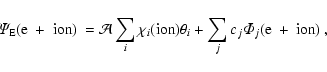
The wavefunction
![]() for the (N+1) electron system with total
spin and orbital angular momenta symmetry
for the (N+1) electron system with total
spin and orbital angular momenta symmetry ![]() or total angular momentum
symmetry
or total angular momentum
symmetry ![]() is expanded in terms of "frozen'' N-electron target ion
functions
is expanded in terms of "frozen'' N-electron target ion
functions ![]() and vector coupled collision electrons
and vector coupled collision electrons ![]() ,
,
 |
(1) |
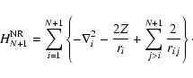
In IP work we restrict the (N+1)-electron Breit-Pauli Hamiltonian to
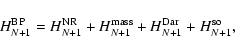 |
(2) |
R-matrix solutions of coupled equations to total symmetries LS are recoupled in a pair coupling scheme on adding spin-orbit interaction
to obtain (
![]() )
states of total
)
states of total ![]() ,
in the end yielding
(N+1)-electron solutions
,
in the end yielding
(N+1)-electron solutions
 |
(5) |
The primary quantity expressing radiative excitation or de-excitation
in a weak field is the line strength
 |
(12) |
 |
(13) |
BPRM calculations span several stages of computation (Berrington et al.
1995). We take radial Fe XVIII wavefuntions from SUPERSTRUCTURE (Eissner
et al. 1974) as input to STG1 to compute Slater, magnetic and
multipole integrals - obtained with Thomas-Fermi scaling parameters
![]() of 1.3835, 1.1506, 1.0837, 1.0564, 1.0175, 1.0390 for
orbitals nl= 1s, 2s, 2p... 3d, which leads to excited levels
2s22p5 2P
of 1.3835, 1.1506, 1.0837, 1.0564, 1.0175, 1.0390 for
orbitals nl= 1s, 2s, 2p... 3d, which leads to excited levels
2s22p5 2P
![]() and 2s2p6 2S1/2 at 0.9403 and 9.8092 Rydbergs above the ground state 2s22p5 2P
and 2s2p6 2S1/2 at 0.9403 and 9.8092 Rydbergs above the ground state 2s22p5 2P
![]() (while including correlation terms from 6 configurations: 2s22p43land 2s2p53l - "1s2'' suppressed for brevity); the excitation
energies above the ground state compare with NIST data of 0.93477 and 9.7023 Ry respectively. Other excited levels of Fe XVIII lie too
high to play a role as parent for any Fe XVII bound states (50 Ry
separating M- from L-shell: level 2s22p43s 4P5/2 at 57.01 Ry), and therefore need not be considered for radiative
calculations. Radial integrals for the partial wave expansion in Eq. (1)
are specified for orbitals
(while including correlation terms from 6 configurations: 2s22p43land 2s2p53l - "1s2'' suppressed for brevity); the excitation
energies above the ground state compare with NIST data of 0.93477 and 9.7023 Ry respectively. Other excited levels of Fe XVIII lie too
high to play a role as parent for any Fe XVII bound states (50 Ry
separating M- from L-shell: level 2s22p43s 4P5/2 at 57.01 Ry), and therefore need not be considered for radiative
calculations. Radial integrals for the partial wave expansion in Eq. (1)
are specified for orbitals
![]() as a basis of NRANG2 =
11 "continuum'' functions - sufficient for bound electrons with n < 10at a radius RA = 2.3750 (Bohr radii a0) of the R-matrix box.
as a basis of NRANG2 =
11 "continuum'' functions - sufficient for bound electrons with n < 10at a radius RA = 2.3750 (Bohr radii a0) of the R-matrix box.
Along with the target description STG2 input specifies which
collisional Fe XVII symmetries LS eventually contribute to
![]() or 8 of even and odd parities, namely
or 8 of even and odd parities, namely
![]() or 8, and multiplicities (2S+1)=1, 3. The second term in Eq. (1), on
bound state correlation functions, is specified to include all possible
(N + 1)-particle configurations from a vacant 2s shell to maximum
occupancies 2s2, 2p6, 3s2, 3p2, and 3d2.
or 8, and multiplicities (2S+1)=1, 3. The second term in Eq. (1), on
bound state correlation functions, is specified to include all possible
(N + 1)-particle configurations from a vacant 2s shell to maximum
occupancies 2s2, 2p6, 3s2, 3p2, and 3d2.
Stage RECUPD transforms to collisional symmetries ![]() or 8
in a pair-coupling representation, and the (e + ion) Hamiltonian R-matrices
for each total
or 8
in a pair-coupling representation, and the (e + ion) Hamiltonian R-matrices
for each total ![]() are diagonalized in STGH employing
observed target energies.
are diagonalized in STGH employing
observed target energies.
In STGB fine structure bound levels are found through the poles
in the (
![]() )
Hamiltonian, searched over a fine mesh of effective
quantum number
)
Hamiltonian, searched over a fine mesh of effective
quantum number ![]() :
:
![]() .
The mesh is orders
of magnitude finer than the typical
.
The mesh is orders
of magnitude finer than the typical
![]() required to find LS energy terms. Intermediate coupling calculations therefore need
orders of magnitude more CPU time than calculations in LS coupling.
Since the fine structure components of higher excited states are more
densely packed, a mesh finer than
required to find LS energy terms. Intermediate coupling calculations therefore need
orders of magnitude more CPU time than calculations in LS coupling.
Since the fine structure components of higher excited states are more
densely packed, a mesh finer than
![]() is essential to
avoid missing any levels.
is essential to
avoid missing any levels.
Table 1:
Comparing effective quantum numbers
![]() of
observed binding energies
of
observed binding energies ![]() with
with
![]() computed in stage
STGB of BPRM (
computed in stage
STGB of BPRM (![]() measured from respective Fe XVIII threshold t). Index IJ counts levels within symmetry
measured from respective Fe XVIII threshold t). Index IJ counts levels within symmetry ![]() in energy order,
* indicating that level J belongs to an incompletely observed multiplet.
in energy order,
* indicating that level J belongs to an incompletely observed multiplet.
Spectroscopically identifying a large number of fine structure levels
poses a major challenge, as the BP Hamiltonian is labelled only by the
total angular momentum and parity, i.e. by ![]() ,
which is
incomplete for unique identification. Complete identification of levels
is needed for various spectral diagnostics and spectrocopic applications
in a lab. A new procedure has been developed and encoded in the
program PRCBPID to identify these levels by a complete set of quantum
numbers through analysis of coupled channels
in the CC expansion (Nahar & Pradhan 2000). This procedure generally
yields unambiguous level identification for most levels. However, for
mixed levels where the identification is to some extent arbitrary, we
assign levels in descending multiplicity (2S+1) and total angular
orbital momentum L. The full
spectroscopic designation reads
,
which is
incomplete for unique identification. Complete identification of levels
is needed for various spectral diagnostics and spectrocopic applications
in a lab. A new procedure has been developed and encoded in the
program PRCBPID to identify these levels by a complete set of quantum
numbers through analysis of coupled channels
in the CC expansion (Nahar & Pradhan 2000). This procedure generally
yields unambiguous level identification for most levels. However, for
mixed levels where the identification is to some extent arbitrary, we
assign levels in descending multiplicity (2S+1) and total angular
orbital momentum L. The full
spectroscopic designation reads
![]() ,
where
,
where ![]() ,
,
![]() ,
,
![]() are the configuration, parent term and
parity, and total angular momentum of target states, nl are the principal
and orbital quantum numbers of the outer or valence electron, and J and
are the configuration, parent term and
parity, and total angular momentum of target states, nl are the principal
and orbital quantum numbers of the outer or valence electron, and J and ![]() are the total angular momentum, term and parity of the
(N+1)-electron system. The procedure also establishes a correspondence
between the fine structure levels and their proper LS terms, and enables
completeness checks to be performed as exemplified below.
are the total angular momentum, term and parity of the
(N+1)-electron system. The procedure also establishes a correspondence
between the fine structure levels and their proper LS terms, and enables
completeness checks to be performed as exemplified below.
STGBB can compute radiative data for transitions of type E1 and E2;
the code exploits methods developed by Seaton (1986) to evaluate the outer
region (>![]() )
contributions to the radiative transition matrix
elements. However, present work reports only E1 transitions from STGBB.
Results for other types of transitions are obtained from SUPERSTRUCTURE, first
optimizing the energy functional over the lowest 49 terms LS (Chen
et al. 2002, CPE02). They arise from 15 configurations: 2s22p6,
2s22p53l, 2s22p54l, 2s12p63l, and 2s12p64l; the
scaling parameters
)
contributions to the radiative transition matrix
elements. However, present work reports only E1 transitions from STGBB.
Results for other types of transitions are obtained from SUPERSTRUCTURE, first
optimizing the energy functional over the lowest 49 terms LS (Chen
et al. 2002, CPE02). They arise from 15 configurations: 2s22p6,
2s22p53l, 2s22p54l, 2s12p63l, and 2s12p64l; the
scaling parameters
![]() for the Thomas-Fermi-Dirac-Amaldi
type potential of orbital nl are listed in Table 1 of CPE02. Much effort
was devoted to choosing scaling parameters to optimise the target
wavefunctions of the M-shell levels. The primary criteria in this
selection are agreement with the observed values for (a) level energies
and fine structure splittings within the lowest terms LS, and (b) f-values for a number of the low lying dipole allowed transitions.
Another practical criterion is that the calculated coefficients A should be variationally stable.
for the Thomas-Fermi-Dirac-Amaldi
type potential of orbital nl are listed in Table 1 of CPE02. Much effort
was devoted to choosing scaling parameters to optimise the target
wavefunctions of the M-shell levels. The primary criteria in this
selection are agreement with the observed values for (a) level energies
and fine structure splittings within the lowest terms LS, and (b) f-values for a number of the low lying dipole allowed transitions.
Another practical criterion is that the calculated coefficients A should be variationally stable.
Experimental energy level differences are employed in the calculation of all types of transition probabilities wherever available, ensuring proper phase space (or energy) factors for f or A; only a small number of Fe XVII levels are spectroscopically observed though.
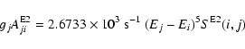
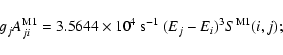
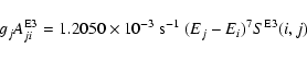
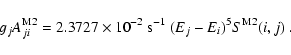
In addition to over 26 000 electric dipole transitions we have
computed
![]() ,
,
![]() ,
,
![]() and
and
![]() for 2312 transitions among the first 89 levels, about half
of these forbidden transition probabilities larger than 103 s-1. Selected transitions (Table 7) are compared with various
other calculations. Results by Safronova et al. (2002, private
communication) are included for comparison.
for 2312 transitions among the first 89 levels, about half
of these forbidden transition probabilities larger than 103 s-1. Selected transitions (Table 7) are compared with various
other calculations. Results by Safronova et al. (2002, private
communication) are included for comparison.
We first describe the BPRM calculations for the energy levels and E1 dipole and intercombination transitions in Fe XVII and then discuss higher multipole order radiation.
A total of 490 bound fine structure energy levels of Fe XVII are obtained
from interacting channels, or Rydberg series
Table 1 tentatively matches the 52 spectroscopically observed levels from NIST with identified levels from our calculations (the level index IJ,
in ascending energy order within a given symmetry ![]() ,
is most useful
for reference in subsequent tables). Calculated effective quantum numbers
,
is most useful
for reference in subsequent tables). Calculated effective quantum numbers
![]() of the first 14 entries differ from observation within
numerical uncertainties and errors due to neglect of two-body magnetic
effects: typically
of the first 14 entries differ from observation within
numerical uncertainties and errors due to neglect of two-body magnetic
effects: typically
![]() .
The abrupt jump
to 0.0027 at level 15 and typical values of 0.002 thereafter can be
explained by the effect of M-shell target levels, for good reasons not
included in the collision type work. For the lowest of the 105 M-shell levels
a structure calculation yields 57.08 Ry above the Fe XVIII ground state;
taking a binding energy of 92.76 Ry for a 2p electron from the first entry in
Table 1, a first quasi-degenerate state can be expected an adequate 35.68 Ry
below the ground state. We see that such homologous states do not seriously
affect the accuracy of our calculation. More important is that M-shell
target configurations do not render it incomplete: a binding energy of
about 40 Ry for a 3s electron taken from entries 2-5 of Table 1 would
lead to true new levels beginning (60-40) Ry above the
ionization limit. It is also worth noting that the quantum defects of these 4 entries are close enough for mere differences
in the Coulomb environment, as s-electrons are not affected by ordinary
spin-orbit coupling. Way down the table agreement deteriorates. While
.
The abrupt jump
to 0.0027 at level 15 and typical values of 0.002 thereafter can be
explained by the effect of M-shell target levels, for good reasons not
included in the collision type work. For the lowest of the 105 M-shell levels
a structure calculation yields 57.08 Ry above the Fe XVIII ground state;
taking a binding energy of 92.76 Ry for a 2p electron from the first entry in
Table 1, a first quasi-degenerate state can be expected an adequate 35.68 Ry
below the ground state. We see that such homologous states do not seriously
affect the accuracy of our calculation. More important is that M-shell
target configurations do not render it incomplete: a binding energy of
about 40 Ry for a 3s electron taken from entries 2-5 of Table 1 would
lead to true new levels beginning (60-40) Ry above the
ionization limit. It is also worth noting that the quantum defects of these 4 entries are close enough for mere differences
in the Coulomb environment, as s-electrons are not affected by ordinary
spin-orbit coupling. Way down the table agreement deteriorates. While
![]() may be considered acceptable and a value 0.01
needs some explanation, the attempts with the 7d and more so 8d levels
are an utter failure, 8d off by 0.13 and 0.04, not to speak of a negative
"observed'' quantum defect of the second 8d level. Such binding energies
may be considered acceptable and a value 0.01
needs some explanation, the attempts with the 7d and more so 8d levels
are an utter failure, 8d off by 0.13 and 0.04, not to speak of a negative
"observed'' quantum defect of the second 8d level. Such binding energies ![]() are unlikely.
are unlikely.
A complete set of energy levels to Fe XVII is available electronically.
As in recent work (e.g. Nahar et al. 2000) the energies are
presented in two formats: (i) in LS term order for spectroscopy and
completeness check, and (ii) in ![]() order for practical applications.
In the term format (i) the fine structure components of a LS term are
grouped together according to the same configuration, useful for
spectroscopic diagnostics. It also checks for completeness
of a set of energy levels that should belong to same LS value
and detects any missing level. Table 2a presents a sample of the table
containing total sets of energies. The table contains partial sets of
levels of Fe XVII. The columns specify the core
order for practical applications.
In the term format (i) the fine structure components of a LS term are
grouped together according to the same configuration, useful for
spectroscopic diagnostics. It also checks for completeness
of a set of energy levels that should belong to same LS value
and detects any missing level. Table 2a presents a sample of the table
containing total sets of energies. The table contains partial sets of
levels of Fe XVII. The columns specify the core
![]() ,
the label nl of the outer electron, total angular momentun J, energy in Rydbergs,
the effective quantum number
,
the label nl of the outer electron, total angular momentun J, energy in Rydbergs,
the effective quantum number ![]() of the valence electron, and possible
term designations LS of the level.
No effective quantum number is assigned to an equivalent electron state.
of the valence electron, and possible
term designations LS of the level.
No effective quantum number is assigned to an equivalent electron state.
Table 2a:
Sample table of fine structure energy levels of Fe XVII as sets of LS term components; ![]() is the core configuration,
is the core configuration,
![]() is the effective quantum number.
is the effective quantum number.
Table 2b:
Calculated Fe XVII fine structure levels, table not extended
to symmetries other than
![]() .
This symmetry has Nlv = 20 levels
below
.
This symmetry has Nlv = 20 levels
below ![]() for the core ground state series: 3 Rydberg series (
for the core ground state series: 3 Rydberg series (![]() measured from the respective series limits, E from the core ground state 2P3/2, the first limit).
measured from the respective series limits, E from the core ground state 2P3/2, the first limit).
The top line of each set in Table 2a gives the number Nlv of expected
fine structure levels, spin and parity of the set (
![]() ), and
the values of L; the total angular quantum numbers J associated with
each L are quoted parenthetically. This line is followed by the set of BPRM energy levels of same configurations. Nlv(c), at the end of
the set, specifies the total number of J-levels obtained. If
), and
the values of L; the total angular quantum numbers J associated with
each L are quoted parenthetically. This line is followed by the set of BPRM energy levels of same configurations. Nlv(c), at the end of
the set, specifies the total number of J-levels obtained. If
![]() for a set, the calculated energy set is complete. Correspondence
of couplings and completeness of levels is established by the program PRCBPID, which detects and prints missing levels. Each level of a set is
further identified by all possible terms LS (specified in the last column
of the set). Multiple LS terms are arranged according to multiplicity (2S+1) and L as mentioned above. It may be noted that levels are
grouped consistently, closely spaced in energies and effective quantum
numbers, confirming proper designation of terms LS. The effective
quantum number (
for a set, the calculated energy set is complete. Correspondence
of couplings and completeness of levels is established by the program PRCBPID, which detects and prints missing levels. Each level of a set is
further identified by all possible terms LS (specified in the last column
of the set). Multiple LS terms are arranged according to multiplicity (2S+1) and L as mentioned above. It may be noted that levels are
grouped consistently, closely spaced in energies and effective quantum
numbers, confirming proper designation of terms LS. The effective
quantum number (![]() )
is expressed up to two significant digits after
the decimal point; the main object is to show the consistency of fine
structure components in the LS grouping. Each level may be assigned to
one or more LS terms in the last column. For a multiple designation
Hund's rule of decreasing multiplicity (2S+1) and L is applied for
further arrangement. One reason for specifying all possible terms is that
the order of calculated and measured energy levels may not exactly match.
Another reason is that
although our term order arrangement may not apply to all cases
for complex ions, it is nonetheless useful in order to establish
completeness of fine structure components of a given LS multiplet.
)
is expressed up to two significant digits after
the decimal point; the main object is to show the consistency of fine
structure components in the LS grouping. Each level may be assigned to
one or more LS terms in the last column. For a multiple designation
Hund's rule of decreasing multiplicity (2S+1) and L is applied for
further arrangement. One reason for specifying all possible terms is that
the order of calculated and measured energy levels may not exactly match.
Another reason is that
although our term order arrangement may not apply to all cases
for complex ions, it is nonetheless useful in order to establish
completeness of fine structure components of a given LS multiplet.
Format (ii) keeps the fine structure levels together as they emerge in the
computational procedure: for a given symmetry ![]() and in energy order as
shown for
and in energy order as
shown for ![]() in Table 2b, which adds up to
in Table 2b, which adds up to
![]() levels, after
the self-explanatory header line. This format should be more convenient
for easy implementation in astrophysical or other plasma modeling codes
requiring large numbers of energy levels and associated transitions.
Here of course we have a set small and transparent enough for assignment
by hand rather than by the new code (note how different spin-orbit
strength is reflected in
the small difference between the quantum defects
levels, after
the self-explanatory header line. This format should be more convenient
for easy implementation in astrophysical or other plasma modeling codes
requiring large numbers of energy levels and associated transitions.
Here of course we have a set small and transparent enough for assignment
by hand rather than by the new code (note how different spin-orbit
strength is reflected in
the small difference between the quantum defects
![]() of the two
series - here we are facing merely p3/2 with t=1 and p1/2with t=2 because of J=0). The levels are identified by core configuration
of the two
series - here we are facing merely p3/2 with t=1 and p1/2with t=2 because of J=0). The levels are identified by core configuration ![]() and level
and level
![]() ,
the outer electron quantum number nl, total J,
energy against the ionization threshold t=1, effective quantum number
,
the outer electron quantum number nl, total J,
energy against the ionization threshold t=1, effective quantum number ![]() associated with the respective series limit t, and a term designation.
associated with the respective series limit t, and a term designation.
The 490 bound fine structure energy levels of Fe XVII give rise to 26 222 dipole allowed and intercombination E1 transitions. The electronically available set contains calculated transition probabilities A, oscillator strengths f, and line strengths Salong with level energies.
A sample subset of transitions, generated by code STGBB, is presented
in Table 3a. The first record of the raw output file
FVALUE specifies the nuclear charge number Z=26, N=9 electrons
in the core ion Fe XVIII, and processing directives (e.g. 0 -
perturbative channel coupling between RA
and ![]() disabled, 1 - Buttle correction activated). The next two
records, headers for the subsequent Fe XVII transition array data, identify this
array as a pair (
disabled, 1 - Buttle correction activated). The next two
records, headers for the subsequent Fe XVII transition array data, identify this
array as a pair (
![]() )
of symmetries
(
)
of symmetries
(![]() for even and =1 for odd parity), here the electric dipole transition
for even and =1 for odd parity), here the electric dipole transition
![]() .
STGB had computed
NJi=20 levels of the
first symmetry (decoded in Table 2b),
NJk=47 to the second, hence
.
STGB had computed
NJi=20 levels of the
first symmetry (decoded in Table 2b),
NJk=47 to the second, hence
![]() subsequent records, each prefaced by a pair Ii and Ik
of level indices (in energy order for the respective symmetry). Their
bound state energies Ei and Ek below the Fe XVIII ground
state are shown in Cols. 3 and 4 in reduced units z2 Ry.
The radiative result in the last three columns are the gf-values of the
transition (see Eq. (8)) in length and velocity form
and the coefficient A for spontaneous emission (derived in the length
form, see Eq. (9)). The signs of gf are in accord
with Eq. (8) and would reverse on swapping the order of symmetries
subsequent records, each prefaced by a pair Ii and Ik
of level indices (in energy order for the respective symmetry). Their
bound state energies Ei and Ek below the Fe XVIII ground
state are shown in Cols. 3 and 4 in reduced units z2 Ry.
The radiative result in the last three columns are the gf-values of the
transition (see Eq. (8)) in length and velocity form
and the coefficient A for spontaneous emission (derived in the length
form, see Eq. (9)). The signs of gf are in accord
with Eq. (8) and would reverse on swapping the order of symmetries ![]() .
Complete spectroscopic identification of the transitions can be
deduced from tables of type 2b.
For the largest listed value, 2.301
.
Complete spectroscopic identification of the transitions can be
deduced from tables of type 2b.
For the largest listed value, 2.301
![]() /s at
/s at
![]() and
associated with excitation energy 60.846 Ry, Table 2b verifies the initial
level as the Fe XVII ground state; we have not presented
the odd-parity J=1 section but can identify Ii=5 as a low lying
state from Tables 1 or 6 as 2s22p53d 1P
and
associated with excitation energy 60.846 Ry, Table 2b verifies the initial
level as the Fe XVII ground state; we have not presented
the odd-parity J=1 section but can identify Ii=5 as a low lying
state from Tables 1 or 6 as 2s22p53d 1P
![]() ;
this transition
reappears in Table 5 with energy-adjusted 2.28(13)/s.
;
this transition
reappears in Table 5 with energy-adjusted 2.28(13)/s.
Table 3b, dealing with the same transition array but taken from standard
STGBB file stgbb.out makes interesting reading about the internal
workings of the R-matrix method, as it details the contributions to the
(unnormalized) radiative transition amplitude D. While the radial wave
solutions associated with small principal quantum numbers like 2 or 3 lie
entirely inside the R-matrix sphere with radius RA, they have most
nodes outside at values
![]() .
The composition of D therefore
changes from dominant interior contributions DI to large outside
portions DA as n and n' increase. Perturbatively computed coupling
contributions DP between the propagation range for DA and infinity
equally increase, to stay only just small enough at n=11 to be neglected as
in Table 2a (IPERT=0) and in fact most large scale calculations (whereas
vital in collisional work!); unlike Buttle contributions DB, which
compensate for the rigid logarithmic boundary condition at RA, their
computation can be fairly time consuming. Especially transition (15, 29) =
(2P1/2 8p 0
.
The composition of D therefore
changes from dominant interior contributions DI to large outside
portions DA as n and n' increase. Perturbatively computed coupling
contributions DP between the propagation range for DA and infinity
equally increase, to stay only just small enough at n=11 to be neglected as
in Table 2a (IPERT=0) and in fact most large scale calculations (whereas
vital in collisional work!); unlike Buttle contributions DB, which
compensate for the rigid logarithmic boundary condition at RA, their
computation can be fairly time consuming. Especially transition (15, 29) =
(2P1/2 8p 0
![]() P1/2 7d 1
P1/2 7d 1![]() reveals a subtle balance among the constituents and between
the amplitudes in length and velocity formulation.
reveals a subtle balance among the constituents and between
the amplitudes in length and velocity formulation.
Table 3a:
Truncated STGBB output " FVALUE'':
gf-values and Einstein coefficients A for [ 0 0 0 0 2 1]
![]() transitions of Fe XVII [ Z=26, core-Nel=9],
as function of bound state energies RE(
transitions of Fe XVII [ Z=26, core-Nel=9],
as function of bound state energies RE(
![]() )
and Re(
)
and Re(
![]() )
in units of z2 Ry, z = 26-9.
The line strength column S(E1) has been added by hand
(see Eqs. (7), (8)) for the first transition array.
)
in units of z2 Ry, z = 26-9.
The line strength column S(E1) has been added by hand
(see Eqs. (7), (8)) for the first transition array.
Table 3b:
Truncated STGBB standard output: array
![]() of Fe XVII, build-up of the dipole transition amplitude
D by the R-matrix code (L[ength] and V[elocity]).
of Fe XVII, build-up of the dipole transition amplitude
D by the R-matrix code (L[ength] and V[elocity]).
Table 4:
Sample set of gf-values and electric dipole
transition probabilities A for Fe XVII in ![]() order. Notation
order. Notation
![]() means
means
![]() .
.
The electronically available compilation of results f, S, and A for
the E1 transitions is formatted differently from Table 3a so as to match
similar files for other ions (e.g. for Fe XXI, Nahar 2000). Table 4
shows what the first section of Table 3a then looks like. The top line retains
the charge number Z but gives ionic
![]() instead of target-N;
the second now assumes intermediate coupling, so
instead of target-N;
the second now assumes intermediate coupling, so
![]() suffices
to specify the transition array
suffices
to specify the transition array
![]() .
The subsequent head line,
starting with the number NJi and NJj of entries for the symmetry pair
just as in Table 3a, names the quantities tabulated for each of the
.
The subsequent head line,
starting with the number NJi and NJj of entries for the symmetry pair
just as in Table 3a, names the quantities tabulated for each of the
![]() transitions. Again the first two columns specify a
transition by level indices i and j, while Rydberg energies of the level
pair are no longer z-scaled. The value
transitions. Again the first two columns specify a
transition by level indices i and j, while Rydberg energies of the level
pair are no longer z-scaled. The value
![]() in Col. 5 is the
quantity GFL of Table 3a (symmetrical in initial and final state: with
statistical weight g=J+1 of the initial level, carrying the minus
sign of
in Col. 5 is the
quantity GFL of Table 3a (symmetrical in initial and final state: with
statistical weight g=J+1 of the initial level, carrying the minus
sign of
![]() if the initial is the upper state!). It is derived
from the primary quantity S as of Eqs. (6), (7) given
in the next column, hence subscript L for length formulation. The
associated coefficient Aji of spontaneous emission trails in Col. 7.
if the initial is the upper state!). It is derived
from the primary quantity S as of Eqs. (6), (7) given
in the next column, hence subscript L for length formulation. The
associated coefficient Aji of spontaneous emission trails in Col. 7.
Line strength results from BPRM are used to compute a set of transition probabilities A and f-values for Fe XVII with observed energy separation in favour of the more uncertain calculated energies, exploiting that S does not depend on level energies (the procedure is commonly employed and was first adopted in NIST compilations). The astrophysical models also in general use the observed transition energies for the relevant f and A data. They are more appropriate for comparison or spectral diagnostics.
Coefficients A and gf-values have been reprocessed for all
the allowed transitions (
![]() )
among the observed levels.
A partial set of these transitions is presented in Table 5. The set,
also available electronically, comprises 342 transitions of Fe XVII.
The reprocessed transitions are moreover
ordered according to configuration C and multiplet LS. This enables
one to obtain the f-values for each multiplet LS and check for
completeness of the associated levels. Completeness however also depends
on the observed set of fine structure levels since the transitions in
the set correspond only to the observed levels (NIST). The LS multiplets
serve various comparisons with other calculations and experiment where
fine structure transitions can not be resolved. The level index Iifor each energy level in the table is given next to the g-value
(e.g. gi: Ii) for a easy pointer to the complete f-file.
)
among the observed levels.
A partial set of these transitions is presented in Table 5. The set,
also available electronically, comprises 342 transitions of Fe XVII.
The reprocessed transitions are moreover
ordered according to configuration C and multiplet LS. This enables
one to obtain the f-values for each multiplet LS and check for
completeness of the associated levels. Completeness however also depends
on the observed set of fine structure levels since the transitions in
the set correspond only to the observed levels (NIST). The LS multiplets
serve various comparisons with other calculations and experiment where
fine structure transitions can not be resolved. The level index Iifor each energy level in the table is given next to the g-value
(e.g. gi: Ii) for a easy pointer to the complete f-file.
BPRM coefficients A are compared with other calculations in Table 6, and
with available NIST data. Safronova et al. (2001) obtained data of E1, E2, M1
and M2 type for transitions 2l-3l' of Fe XVII using relativistic many-body
perturbation theory (MBPT). Present results agree reasonably well yet with
noticeable scatter compared to and also within (a)-(e), in particular for
the decay of level 17 (for labels see Table 7):
2s22p53d 3P
![]() 2s22p6 1S0. Because of poorer
consistency for intercombination transitions - as would
happen when varying the strength of multiplet mixing - one might go for
inclusion of all magnetic interactions among the valence electrons: after all
there are 8 of them in this sequence, while BPRM ignores magnetic 2-body
contributions (accounting only for interaction with the two closed-shell 1s
electrons). The result marked by
2s22p6 1S0. Because of poorer
consistency for intercombination transitions - as would
happen when varying the strength of multiplet mixing - one might go for
inclusion of all magnetic interactions among the valence electrons: after all
there are 8 of them in this sequence, while BPRM ignores magnetic 2-body
contributions (accounting only for interaction with the two closed-shell 1s
electrons). The result marked by ![]() looks encouraging - until one
repeats the same short calculation without such terms:
looks encouraging - until one
repeats the same short calculation without such terms:
![]() /s
looks sobering besides the tabulated
/s
looks sobering besides the tabulated
![]() /s. This way Bhatia
& Doschek's (1992) coefficient falls into place, leaving the Cornille et al.
result - also from SUPERSTRUCTURE- the odd case out. The blanks for Cornille
et al. in the last two transitions are not incidental, since they did not
include configurations 2s2p63l which become degenerate to 2s22p53l' in the high Z limit, according to Layzer's scaling laws
(Layzer 1959), that it is essential to include all the configurations of
the complex in order to correctly reproduce the terms of the Z-expansion
of the non-relativistic energy. FS splitting of course is a different matter,
and if 2-body magnetic interaction with the closed K shell is omitted the
effective spin-orbit parameter
/s. This way Bhatia
& Doschek's (1992) coefficient falls into place, leaving the Cornille et al.
result - also from SUPERSTRUCTURE- the odd case out. The blanks for Cornille
et al. in the last two transitions are not incidental, since they did not
include configurations 2s2p63l which become degenerate to 2s22p53l' in the high Z limit, according to Layzer's scaling laws
(Layzer 1959), that it is essential to include all the configurations of
the complex in order to correctly reproduce the terms of the Z-expansion
of the non-relativistic energy. FS splitting of course is a different matter,
and if 2-body magnetic interaction with the closed K shell is omitted the
effective spin-orbit parameter
![]() Ry (0.1484
Ry (0.1484 ![]() /cm) goes up to the "bare'' value of 0.684 Ry (or 0.1644
/cm) goes up to the "bare'' value of 0.684 Ry (or 0.1644 ![]() /cm);
for the effective spin-orbit parameter
/cm);
for the effective spin-orbit parameter ![]() to orbitals l, see Blume &
Watson (1962), Eissner et al. (1974), also Eq. (4).
So much about a mute point of interpreting scatter. For electric
dipole transitions the BPRM code in its present state is as good as other good
approaches but readily delivering far larger data sets than anything to date.
to orbitals l, see Blume &
Watson (1962), Eissner et al. (1974), also Eq. (4).
So much about a mute point of interpreting scatter. For electric
dipole transitions the BPRM code in its present state is as good as other good
approaches but readily delivering far larger data sets than anything to date.
Among forbidden transitions, discussed in the next section, there is one class for which it is obvious that one must draw very different conclusions, that is for transitions between levels of a FS multiplet: to start with, the splitting changes significantly on including 2-body FS contributions.
Table 5:
Dipole allowed and intercombination transitions in Fe XVII.
The calculated transition energies are replaced by observed energies.
The g:I indices refer to the statistical weight:energy level index in the
raw data file. The notation a(b) means
![]() .
.
We extend the behavioural study of computed radiative decay in Table 8
to a selection of forbidden transitions; a complete set
will be published in electronic format, available from the CDS library
for 2312 transitions between the 89 Fe XVII-levels. Table 8 along
with Table 7 probes the quality of the target representations -
especially term coupling, which is crucial in the
collisional application (CPE02). Larger uncertainties are confined to
intercombination lines, but there they can increase uncomfortably with
higher radiative multipole type. Moreover the table assesses the
influence of 2-body finestructure contributions neglected in the current
BPRM work. Magnetic interaction between valence shell electrons is
always present in the MCDF work with GRASP, activated for the
SUPERSTRUCTURE column SS![]() but switched
off in SS
but switched
off in SS![]() :
follow the trend from SS
:
follow the trend from SS![]() via SS
via SS![]() to full relativistic MCDF.
to full relativistic MCDF.
At wave lengths of 10 Å ![]() 911 Å/100 (hence
Eij2=104 Ry) Eqs. (16), (17) versus (14), (15) suggest a close look at decay by electric octopole and
magnetic quadrupole radiation for transitions with such a
lowest path. We can indeed expect rates around 106/s, which would be
competitive with E2 and M1 decay around Fe with
911 Å/100 (hence
Eij2=104 Ry) Eqs. (16), (17) versus (14), (15) suggest a close look at decay by electric octopole and
magnetic quadrupole radiation for transitions with such a
lowest path. We can indeed expect rates around 106/s, which would be
competitive with E2 and M1 decay around Fe with
![]() along
the Ne-isoelectronic sequence, as the scaling laws show: inserting (7) for E
along
the Ne-isoelectronic sequence, as the scaling laws show: inserting (7) for E![]() and (11) for M
and (11) for M![]() into the line
strength expression (6) yields scaling of A as Z8 for both E3 and M2 (and Z6 for E2 and M1); for transitions within a principal shell
(
into the line
strength expression (6) yields scaling of A as Z8 for both E3 and M2 (and Z6 for E2 and M1); for transitions within a principal shell
(
![]() )
though scaling of E
)
though scaling of E![]() drops by a factor of Z2, and
octopole transitions become negligible; we do not extend this discussion to
intercombination transitions. The E3 results in Table 8 are most
satisfactory and perfectly understood. To start with the two bottom entries,
one of them apparently contradicting this statement, Table 7 identifies levels 87 and 89 as multiplet mixing companions with J=3 to terms 4f3F
and 1F. Therefore the intercombination decay of 87 becomes rather
sensitive to magnetic coupling, A converging from right to left as much
as one can reasonably expect when MCDF works with a slightly different
target. This is borne out by 56, the only other troubling level for E3,
as Table 7 places it marginally differently (unfortunately no experiment has
yet decided). M2 is a different matter, a factor of 2.5 in the poor case (18,1) difficult to reconcile with the lowest order radiative operator as
adopted in SUPERSTRUCTURE.
drops by a factor of Z2, and
octopole transitions become negligible; we do not extend this discussion to
intercombination transitions. The E3 results in Table 8 are most
satisfactory and perfectly understood. To start with the two bottom entries,
one of them apparently contradicting this statement, Table 7 identifies levels 87 and 89 as multiplet mixing companions with J=3 to terms 4f3F
and 1F. Therefore the intercombination decay of 87 becomes rather
sensitive to magnetic coupling, A converging from right to left as much
as one can reasonably expect when MCDF works with a slightly different
target. This is borne out by 56, the only other troubling level for E3,
as Table 7 places it marginally differently (unfortunately no experiment has
yet decided). M2 is a different matter, a factor of 2.5 in the poor case (18,1) difficult to reconcile with the lowest order radiative operator as
adopted in SUPERSTRUCTURE.
For E2 vs. M1 the picture turns very varied as early as for
![]() :
distinguishing between intercombination transitions (with factors
like
:
distinguishing between intercombination transitions (with factors
like
![]() and
and
![]() )
and direct transition becomes a more
persistent companion. For direct transitions between main shells both A scale as Z6, the time coefficient favouring E2. Next come radiative BP corrections to M1 remembered from the classical case of 1s2s 3S decay.
We verified the Bhatia and Doschek entries, converting to A without those
corrections with the help of an expedient tool: SUPERSTRUCTURE prints both the full
line strength
)
and direct transition becomes a more
persistent companion. For direct transitions between main shells both A scale as Z6, the time coefficient favouring E2. Next come radiative BP corrections to M1 remembered from the classical case of 1s2s 3S decay.
We verified the Bhatia and Doschek entries, converting to A without those
corrections with the help of an expedient tool: SUPERSTRUCTURE prints both the full
line strength
![]() and BP-deficient
and BP-deficient
![]() .
Then A(9,1) drops to less than its tenth, from its SS
.
Then A(9,1) drops to less than its tenth, from its SS![]() result
result
![]() s-1 - albeit only half what MCDF is telling: greater discrepancies are
associated with differences between SS
s-1 - albeit only half what MCDF is telling: greater discrepancies are
associated with differences between SS![]() and SS
and SS![]() results and rather
crowded fields in Table 7 for the respective
results and rather
crowded fields in Table 7 for the respective ![]() ,
so BP may be stretched
beyond its limits. The trends for E2 type transitions look perfect.
,
so BP may be stretched
beyond its limits. The trends for E2 type transitions look perfect.
For electric dipole transitions, both direct and spin-flip, Table 8 gives Ain velocity form as a second entry to the more firmly established length results, as a measure of good target description (with the proviso after Eq. (7)). They compare encouragingly for the EIE work.
Table 6:
Comparison of BPRM calculations for decay
![]() to the Fe XVII ground state C1T1 = 2s22p6 1S0with other work.
to the Fe XVII ground state C1T1 = 2s22p6 1S0with other work.
Turning briefly towards astrophysical and laboratory implications from Table 8, apart from selected spontaneous emission coefficients for dipole-allowed transitions it gives results for magnetic dipole and electric quadrupole radiation - and some magnetic quadrupole and electric octopole transitions of the same magnitude of some 106 s-1: of course this high multipole decay mode can compete only for transitions with very short wave length, i.e. to the ground state. It may influence the modeling of line emissions. In astronomy and in laboratory photoionized plasmas the M2 decay from level 2 has long been observed as a prominent line. The population of level 2 is fed by cascading from 2p53s, 2p53p, and 2p53d and higher configurations. Accurate M2 transition probabilities are the key to modeling this line. Moreover it has important plasma diagnostics potential.
From large-scale state-of-the-art calculations in Breit-Pauli approximation we obtain energy levels with principal quantum number up to n=10 and radiative transition probabilities of Fe XVII. All levels have been identified in spectroscopic notation and checked for completeness. The set of results far exceeds the currently available experimental and theoretical data.
Radiative data for most electric dipole transions as well as level positions agree within 10% and in most cases far better with available theoretical and experimental work of quality. This indicates that for these highly charged ions higher order relativistic and QED effects omitted in the BPRM calculations may lead to an error not exceeding the estimated uncertainty.
We have obtained a consistent set of coefficients A for E2 and M1 type
transitions and compared our SUPERSTRUCTURE and MCDF calculations with other
calculations in the literature. Most results for
![]() and
and
![]() lie well inside 20-30% of uncertainty. However, numerically very small
coefficients can differ from 50% to a factor of two: M2 and in particular E3 results are highly sensitive to the physics included and numerics (e.g. cancellation effects and numerical instabilities). Large differences are found
between the SUPERSTRUCTURE and MCDF calculations. Especially the magnetic quadrupole
results are hard to assess, suggesting further study of this issue.
lie well inside 20-30% of uncertainty. However, numerically very small
coefficients can differ from 50% to a factor of two: M2 and in particular E3 results are highly sensitive to the physics included and numerics (e.g. cancellation effects and numerical instabilities). Large differences are found
between the SUPERSTRUCTURE and MCDF calculations. Especially the magnetic quadrupole
results are hard to assess, suggesting further study of this issue.
Table 7:
The first 89 fine-structure n=2, 3 and 4 levels included in
the EIE calculation by Chen et al. 2003: comparison of calculated and
observed energies in Rydbergs for Fe XVII; "obs'' data are observed
values from NIST; the entries " SS'' ( SS![]() / SS
/ SS![]() :
without/with inclusion of 2-body magnetic components) and the entries
" MCDF'' are from SUPERSTRUCTURE and GRASP calculations respectively.
:
without/with inclusion of 2-body magnetic components) and the entries
" MCDF'' are from SUPERSTRUCTURE and GRASP calculations respectively.
Table 8:
Selected transition probabilities ![]() s of Fe XVII, for electric dipole E1 type transitions also in velocity
formulation as second entries, computed by SUPERSTRUCTURE with and without
2-body FS-terms (columns SS
s of Fe XVII, for electric dipole E1 type transitions also in velocity
formulation as second entries, computed by SUPERSTRUCTURE with and without
2-body FS-terms (columns SS![]() and SS
and SS![]() )
and MCDF, and miscellaneous results: E1 - from BPRM,
M1 -
)
and MCDF, and miscellaneous results: E1 - from BPRM,
M1 -
![]() s by Bhatia & Doschek (1992)
employing (11) rather than full (10),
E2 - from BPRM.
The quantity aeb stands for
s by Bhatia & Doschek (1992)
employing (11) rather than full (10),
E2 - from BPRM.
The quantity aeb stands for
![]() .
.
All data are available electronically. Part of the f-values have been reprocessed using available observed energies for better accuracy. The new results should be particularly useful for the analysis of X-ray and Extreme Ultraviolet spectra from astrophysical and laboratory sources where non-local thermodynamic equilibrium (NLTE) atomic models with many excited levels are needed.
Acknowledgements
This work was partially supported by U.S. National Science Foundation (AST-9870089) and the NASA ADP program; WE enjoyed part-support by Sonderforschungsbereich 392 of the German Research Council. The computational work was largely carried out on the Cray T94 and Cray SV1 at the Ohio Supercomputer Center in Columbus, Ohio.
![\begin{displaymath}O^{{\rm E}\lambda} = b^{[\lambda]}\sum_{p=1}^{N+1}
{\rm C}^{...
..., \qquad\quad
b^{[\lambda]} = \sqrt{\frac{2}{\lambda+1}}\cdot
\end{displaymath}](/articles/aa/full/2003/35/aa3648/img53.gif)
![\begin{displaymath}O^{{\rm M}\lambda} = b^{[\lambda]}\sum_pr_p^{\lambda-1}\Big[
...
...mes\big\{
{l}(p)+(\lambda+1){s}(p)\big\}\Big]^{[\lambda]}\!.~
\end{displaymath}](/articles/aa/full/2003/35/aa3648/img65.gif)