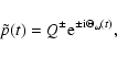
According to Eq. (20),
 |
(71) |
 |
(72) |
 |
(73) |
| |
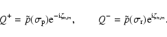
= | (74a) | |
| = | (74b) |
| Q- | = | (75a) | |
| Fn,0(-) | = | (75b) |
| Forcing | Coefficients in
|
Coefficients in
|
||
| potential |
|
|
|
|
| Prograde polar motions | ||||
| (2, 1) | C2,2 | S2,2 | -S2,2 | C2,2 |
| (3, 0) | -C3,1 | -S3,1 | S3,1 | -C3,1 |
| (3, 1) | -S3,2 | C3,2 | -C3,2 | -S3,2 |
| (3, 2) | -C3,3 | -S3,3 | S3,3 | -C3,3 |
| (4, 0) | S4,1 | -C4,1 | C4,1 | S4,1 |
| (4, 1) | C4,2 | S4,2 | -S4,2 | C4,2 |
| Retrograde polar motions | ||||
| (3, 0) | -C3,1 | S3,1 | S3,1 | C3,1 |
| (3, 2) | C3,1 | S3,1 | S3,1 | -C3,1 |
| (3, 3) | S3,2 | -C3,2 | -C3,2 | -S3,2 |
| (4, 0) | -S4,1 | -C4,1 | -C4,1 | S4,1 |
We have carried out the numerical evaluation of the coefficients of
polar motions due to tidal potentials of degrees up to 4,
starting from the tidal amplitudes defined according to the
conventions of
Cartwright & Tayler (1971).
Actually, we used
the RATGP series of Roosbeek (1996) and converted the amplitudes
from this series to their Cartwright-Tayler equivalents through
multiplication by the appropriate factors fn,m taken from
Table 6.5 of the IERS Conventions 1996. (The sign of the factor f3,1 given there has to be reversed; the
value
f4,0= 0.317600 not listed there was
needed to compute polar motions with coefficients down to 0.05 ![]() as,
there being a few that are excited by
(4, 0) potentials.)
For the prograde diurnal polar motions, we have also used the
alternative approach explained in Sect. 7, using the known
amplitudes of the long period nutations as inputs instead of the
tidal amplitudes. The JGM3 values listed in Table 2 were used for the
geopotential coefficients in computations for the nonrigid Earth;
the IERS92 values were used for the rigid Earth case, to
facilitate comparisons with the results of earlier workers.
as,
there being a few that are excited by
(4, 0) potentials.)
For the prograde diurnal polar motions, we have also used the
alternative approach explained in Sect. 7, using the known
amplitudes of the long period nutations as inputs instead of the
tidal amplitudes. The JGM3 values listed in Table 2 were used for the
geopotential coefficients in computations for the nonrigid Earth;
the IERS92 values were used for the rigid Earth case, to
facilitate comparisons with the results of earlier workers.
We present in Table 4 the periodic polar
motions having amplitudes exceeding 0.5 ![]() as. Only the low
frequency polar motions due to (3, 0) potentials and the prograde
diurnals excited by the (2, 1) potentials attain these
magnitudes. The secular polar motion due to the constant term in
the (4, 0) potential is also shown. The argument of the polar motion,
denoted by (arg) in the Table, is
as. Only the low
frequency polar motions due to (3, 0) potentials and the prograde
diurnals excited by the (2, 1) potentials attain these
magnitudes. The secular polar motion due to the constant term in
the (4, 0) potential is also shown. The argument of the polar motion,
denoted by (arg) in the Table, is
![]() if the motion is
prograde, and
if the motion is
prograde, and
![]() if retrograde. It is expressed here as a
linear combination,
if retrograde. It is expressed here as a
linear combination,
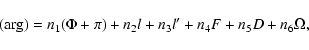 |
(76) |
The argument of the HF nutation equivalent to the polar motion of (76) is
| (77) |
| n | Multipliers of | Period |
|
|
Nutation | |||||||
| l | l' | F | D | of PM | Period | |||||||
| 3 | 0 | -1 | 0 | -1 | 0 | -1 | -13.719 | 1.39 | .17 | -.17 | 1.39 | 1.07545 |
| 3 | 0 | 0 | 0 | -1 | 0 | 0 | -27.212 | 2.48 | .30 | -.30 | 2.48 | 1.03521 |
| 3 | 0 | 0 | 0 | -1 | 0 | -1 | -27.322 | 15.75 | 1.93 | -1.93 | 15.75 | 1.03505 |
| 3 | 0 | 0 | 0 | -1 | 0 | -2 | -27.432 | -.82 | -.10 | .10 | -.82 | 1.03489 |
| 3 | 0 | -1 | 0 | -1 | 2 | -1 | -193.560 | .81 | .10 | -.10 | .81 | 1.00243 |
| 3 | 0 | 1 | 0 | -1 | 0 | 0 | -2190.35 | 1.86 | .24 | -.24 | 1.86 | .99772 |
| 3 | 0 | 1 | 0 | -1 | 0 | -1 | -3231.50 | 12.32 | 1.59 | -1.59 | 12.32 | .99758 |
| 3 | 0 | 1 | 0 | -1 | 0 | -2 | -6159.14 | -.68 | -.09 | .09 | -.68 | .99743 |
| 3 | 0 | -1 | 0 | 1 | 0 | 2 | 6159.14 | .78 | .09 | -.09 | .78 | .99711 |
| 3 | 0 | -1 | 0 | 1 | 0 | 1 | 3231.50 | -16.16 | -1.83 | 1.83 | -16.16 | .99696 |
| 3 | 0 | -1 | 0 | 1 | 0 | 0 | 2190.35 | -2.78 | -.31 | .31 | -2.78 | .99682 |
| 3 | 0 | 1 | 1 | -1 | 0 | 0 | 438.360 | -.63 | .12 | -.12 | -.63 | .99501 |
| 3 | 0 | 1 | 1 | -1 | 0 | -1 | 411.807 | 1.05 | .27 | -.27 | 1.05 | .99486 |
| 3 | 0 | 0 | 0 | 1 | -1 | 1 | 365.242 | 1.31 | .20 | -.20 | 1.31 | .99455 |
| 3 | 0 | 1 | 0 | 1 | -2 | 1 | 193.560 | 2.10 | .27 | -.27 | 2.10 | .99216 |
| 3 | 0 | 0 | 0 | 1 | 0 | 2 | 27.432 | -.87 | -.11 | .11 | -.87 | .96229 |
| 3 | 0 | 0 | 0 | 1 | 0 | 1 | 27.322 | 16.64 | 2.04 | -2.04 | 16.64 | .96215 |
| 3 | 0 | 0 | 0 | 1 | 0 | 0 | 27.212 | 2.62 | .32 | -.32 | 2.62 | .96201 |
| 3 | 0 | 1 | 0 | 1 | 0 | 1 | 13.719 | 1.28 | .16 | -.16 | 1.28 | .92969 |
| 2 | 1 | -1 | 0 | -2 | 0 | -1 | 1.11970 | -.44 | .25 | -.25 | -.44 | .52747 |
| 2 | 1 | -1 | 0 | -2 | 0 | -2 | 1.11951 | -2.31 | 1.32 | -1.32 | -2.31 | .52743 |
| 2 | 1 | 1 | 0 | -2 | -2 | -2 | 1.11346 | -.44 | .25 | -.25 | -.44 | .52608 |
| 2 | 1 | 0 | 0 | -2 | 0 | -1 | 1.07598 | -2.14 | 1.23 | -1.23 | -2.14 | .51756 |
| 2 | 1 | 0 | 0 | -2 | 0 | -2 | 1.07581 | -11.36 | 6.52 | -6.52 | -11.36 | .51753 |
| 2 | 1 | -1 | 0 | 0 | 0 | 0 | 1.03472 | .84 | -.48 | .48 | .84 | .50782 |
| 2 | 1 | 0 | 0 | -2 | 2 | -2 | 1.00275 | -4.76 | 2.73 | -2.73 | -4.76 | .50000 |
| 2 | 1 | 0 | 0 | 0 | 0 | 0 | .99727 | 14.27 | -8.19 | 8.19 | 14.27 | .49863 |
| 2 | 1 | 0 | 0 | 0 | 0 | -1 | .99712 | 1.93 | -1.11 | 1.11 | 1.93 | .49860 |
| 2 | 1 | 1 | 0 | 0 | 0 | 0 | .96244 | .76 | -.43 | .43 | .76 | .48977 |
| Rate of secular polar motion ( |
||||||||||||
| 4 | 0 | 0 | 0 | 0 | 0 | 0 | -3.80 | -4.31 | .99727 | |||
The coefficients of the HF nutations may be inferred from those of the equivalent polar motions from the following considerations.
Beginning with the fact that
![]() ,
which
produces an overall sign difference between the
coefficients of
,
which
produces an overall sign difference between the
coefficients of
![]() and
and
![]() in
in
![]() and
and
![]() ,
on the one hand, and those of
,
on the one hand, and those of
![]() and
and
![]() in
in
![]() and
and
![]() on the other hand, one takes note of the other sign differences
that occur: a sign (-1)m depending on the order m of the tidal
potential giving rise to the motions, which arises from the
relations (15) between
on the other hand, one takes note of the other sign differences
that occur: a sign (-1)m depending on the order m of the tidal
potential giving rise to the motions, which arises from the
relations (15) between
![]() and
and
![]() ,
and a further
minus sign that arises between the coefficients in
,
and a further
minus sign that arises between the coefficients in
![]() on the one hand and those in
on the one hand and those in
![]() on the other
because of the fact that
on the other
because of the fact that
![]() while
while
![]() .
Thus, with
superscripts s and c identifying coefficients of the sine and
cosine functions, respectively, of (arg) or
.
Thus, with
superscripts s and c identifying coefficients of the sine and
cosine functions, respectively, of (arg) or ![]() as the case
may be, we have
as the case
may be, we have
| (78a) | |||
| (78b) |
The above relations, when combined with (73), show that the coeffients
of any circular polar motion and of the corresponding nutation can all
be obtained from just two of them, say
![]() and
and
![]() .
They
supersede Eqs. (24) of Mathews & Bretagnon (2002)
which fail to be valid in general as the sign factors referred to
below Eq. (17) were overlooked.
.
They
supersede Eqs. (24) of Mathews & Bretagnon (2002)
which fail to be valid in general as the sign factors referred to
below Eq. (17) were overlooked.
Our results for a few of the leading terms in the semidiurnal
nutations due to degree 2 potentials, which are strictly prograde
and hence circular, are compared with the results from earlier
works in Table 5. The coefficients
![]() and
and
![]() are
shown both for the rigid and the nonrigid Earth;
are
shown both for the rigid and the nonrigid Earth;
![]() and
and
![]() in the
present case. The values shown against BCpc were obtained by
conversion from recent polar motion coefficients of
Brzezinski & Capitaine
(private communication, 2002).
Elliptical nutations (including semidiurnal ones) that are induced
by higher degree potentials are considered below.
in the
present case. The values shown against BCpc were obtained by
conversion from recent polar motion coefficients of
Brzezinski & Capitaine
(private communication, 2002).
Elliptical nutations (including semidiurnal ones) that are induced
by higher degree potentials are considered below.
| Period | Rigid Earth | Nonrigid Earth | ||||
| (days) | Authors |
|
|
Authors |
|
|
| 0.51753 | BRS97 | 5.79 | 10.09 | GFE01 | 6.54 | 11.39 |
| FBS01 | 5.8 | 10.0 | FBS01 | 6.5 | 11.3 | |
| BCpc | 5.83 | 10.16 | BCpc | 6.57 | 11.45 | |
| Present | 5.87 | 10.22 | Present | 6.52 | 11.36 | |
| 0.50000 | BRS97 | 2.43 | 4.23 | GFE01 | 2.74 | 4.77 |
| FBS01 | 2.37 | 4.13 | FBS01 | 2.7 | 4.7 | |
| BCpc | 2.44 | 4.25 | BCpc | 2.75 | 4.79 | |
| Present | 2.46 | 4.28 | Present | 2.73 | 4.76 | |
| 0.49863 | BRS97 | -7.27 | -12.67 | GFE01 | -8.21 | -14.30 |
| FBS01 | -7.12 | -12.40 | FBS01 | -8.0 | -14.0 | |
| BCpc | -7.32 | -12.75 | BCpc | -8.25 | -14.37 | |
| Present | -7.27 | -12.67 | Present | -8.19 | -14.27 | |
|
a BRS97: Bretagnon et al. (1997); FBS01:
Folgueira et al. (2001); GFE01: Getino et al. (2001); and BCpc: Brzezinski & Capitaine (private communication, 2002). |
| Type of | Period (days) of | Coefficients | ||||
| Tide | Wobble | Nutation |
|
|
|
|
| Diurnal nutations | ||||||
| (3,0) | -27.322 | 1.03505 | -34.201 | -4.204 | -1.672 | 13.604 |
| (3,2) | -.50790 | -1.03505 | .604 | -.074 | -.030 | -.240 |
| Total | -34.805 | -4.278 | -1.642 | 13.364 | ||
| BRS97 | -34.821 | -4.271 | -1.640 | 13.371 | ||
| FBS01 | -35.404 | -4.351 | -1.587 | 12.911 | ||
| (3,0) | -3231.5 | .99758 | -19.881 | -2.444 | -.972 | 7.908 |
| (3,2) | -.49871 | -.99758 | .031 | -.004 | -.002 | -.012 |
| Total | -19.912 | -2.448 | -.970 | 7.896 | ||
| BRS97 | -19.854 | -2.491 | -.988 | 7.873 | ||
| FBS01 | -19.940 | -2.451 | -.972 | 7.906 | ||
| (3,0) | 27.322 | .96215 | -38.080 | -4.680 | -1.862 | 15.147 |
| (3,2) | -.48970 | -.96215 | .050 | -.006 | -.002 | -.020 |
| Total | -38,130 | -4.686 | -1.860 | 15.127 | ||
| BRS97 | -38.128 | -4.695 | -1.863 | 15.127 | ||
| FBS01 | -38.231 | -4.699 | -1.857 | 15.106 | ||
| Semidiurnal nutations | ||||||
| (3,1) | .89050 | .527517 | -.074 | -.108 | -.043 | .029 |
| (3,3) | -2.89050 | -.527517 | .106 | -.154 | -.061 | -.042 |
| Total | -.180 | -.262 | .018 | -.013 | ||
| BRS97 | -.178 | -.258 | .020 | -.013 | ||
| FBS01 | -.109 | -.388 | .234 | -.092 | ||
| (3,1) | .963499 | .507904 | -.206 | -.301 | -.120 | .082 |
| (3,3) | -2.963499 | -.507904 | .013 | -.019 | -.008 | -.005 |
| Total | -.219 | -.320 | -.112 | .077 | ||
| BRS97 | -.219 | -.321 | -.113 | .077 | ||
| FBS01 | -.244 | -.356 | -.097 | .067 | ||
The combination of two circular motions differing only in the sign
of the frequency describes an elliptical motion. In Table 4,
such prograde-retrograde pairs of terms appear only among the low
frequency polar motions. The argument
![]() of the prograde part is
assigned to the elliptical polar motion. Since
of the prograde part is
assigned to the elliptical polar motion. Since
![]() for
the retrograde part, the signs of the coefficients in the sine
columns have to be reversed in the row pertaining to any retrograde
PM before adding to the coefficients in the row pertaining to the
corresponding prograde PM to obtain the coefficients for the
elliptical motion.
For the elliptical PM with the 27.322 day period, for
instance, one finds the coefficients (in the same order as in the
table) to be (
0.89, 3.99, -0.11, 32.35)
for
the retrograde part, the signs of the coefficients in the sine
columns have to be reversed in the row pertaining to any retrograde
PM before adding to the coefficients in the row pertaining to the
corresponding prograde PM to obtain the coefficients for the
elliptical motion.
For the elliptical PM with the 27.322 day period, for
instance, one finds the coefficients (in the same order as in the
table) to be (
0.89, 3.99, -0.11, 32.35) ![]() as; they are (
-28.49,
-0.24, 3.44, -3.85)
as; they are (
-28.49,
-0.24, 3.44, -3.85) ![]() as for the 3231.496 day polar motion. Note
the predominance of the cosine part of
as for the 3231.496 day polar motion. Note
the predominance of the cosine part of ![]() in the former case and
of the sine part of
in the former case and
of the sine part of ![]() in the latter. The difference in
behaviour is due to the presence of the Chandler mode in between
these periods.
in the latter. The difference in
behaviour is due to the presence of the Chandler mode in between
these periods.
For higher frequency PM, (e.g., the semidiurnals), the
prograde and retrograde parts originate in the action of the
same potential on different geopotential coefficients, e.g.,
by the action of (3, 2) potentials on C3,3 and S3,3 for
prograde semidiurnals, and on C3,1 and S3,1 for the
retrograde ones. The largest of these, with periods of +0.52752and -0.52752 have coefficients (
-0.330, -.0041, -0.041,
0.330) and (
-0.028,-0.055,0.055,-0.028) ![]() as, respectively; both
sets are below the cuf-off for inclusion in Table 4. The elliptical
motion from their combination has coefficients (
-0.358, -0.096, 0.014,
0.302)
as, respectively; both
sets are below the cuf-off for inclusion in Table 4. The elliptical
motion from their combination has coefficients (
-0.358, -0.096, 0.014,
0.302) ![]() as.
as.
In contrast to elliptical polar motions, elliptical HF nutations
result from the combination of a pair of prograde and retrograde
nutations produced by different potentials acting on the same C and S coefficients. It must be noted that the semidiurnal
nutations arising from the action of degree 2 potentials on C2,2
and S2,2 are strictly prograde and circular: there exists no (2, 3) potential to generate retrograde components. Thus the elliptical
nutations are generated only by higher degree potentials. Table 6
shows a few examples from our computations for the rigid Earth, and
comparisons with the results of Bretagnon et al. (1997) and
Folgueira et al. (2001) - both of which are for elliptical
nutations only. Since both these works have employed
the values listed under IERS92 in Table 2 for Cn,m and Sn,m, our numbers used for the comparison are based on the
same values. The ratios
![]() and
and
![]() should be equal to
(-C3,1/S3,1) for the diurnal nutations and
(S3,2/C3,2) for the semidiurnals, as may be seen from our
theory. This requirement is satisfied rather well by all the sets of
coefficients shown, except those of Folgueira et al. (2001)
for the 0.527517 day nutation which are inconsistent with the above
requirement. In fact, the fractional differences of their
numbers from ours are not really small for the other listed
semidiurnals too. Our sets of values are very close to those of
Bretagnon et al.; and for the diurnal nutations, they are
quite close to Folgueira et al. too.
should be equal to
(-C3,1/S3,1) for the diurnal nutations and
(S3,2/C3,2) for the semidiurnals, as may be seen from our
theory. This requirement is satisfied rather well by all the sets of
coefficients shown, except those of Folgueira et al. (2001)
for the 0.527517 day nutation which are inconsistent with the above
requirement. In fact, the fractional differences of their
numbers from ours are not really small for the other listed
semidiurnals too. Our sets of values are very close to those of
Bretagnon et al.; and for the diurnal nutations, they are
quite close to Folgueira et al. too.
The coefficients shown in Table 4 for the prograde diurnal polar
motions do not take account of possible triaxiality of the core.
How much of a difference could core triaxiality make? To answer
this question, we have made computations based on Eqs. (64)
with nonzero ![]() as well as with
as well as with
![]() ,
and taken the
difference. To facilitate comparison with the results of
Escapa et al. (2002), we present in Table 7 our results for the
contributions from
,
and taken the
difference. To facilitate comparison with the results of
Escapa et al. (2002), we present in Table 7 our results for the
contributions from ![]() to the equivalent semidiurnal nutations
when
to the equivalent semidiurnal nutations
when
![]() ,
together with numbers from the IT columns
of Table 1 of their paper which pertain to the same ratio for
,
together with numbers from the IT columns
of Table 1 of their paper which pertain to the same ratio for
![]() which is, in their notation,
which is, in their notation,
![]() .
Only the
coefficients of the increment
.
Only the
coefficients of the increment
![]() due to
due to ![]() are
shown. It is evident that the Escapa et al. values are 2.4 to 3 times as large as ours, except for the .51753 day nutation
for which the factor is nearly 8. We have not been able to
discern the reason for the discrepancies; and we find no scope
for modifying our expressions to bridge the gap, our derivations
being entirely transparent.
are
shown. It is evident that the Escapa et al. values are 2.4 to 3 times as large as ours, except for the .51753 day nutation
for which the factor is nearly 8. We have not been able to
discern the reason for the discrepancies; and we find no scope
for modifying our expressions to bridge the gap, our derivations
being entirely transparent.
| Nutation perioda | Present work | Escapa et al. | |||
| PSD | LF |
|
|
|
|
| .49863 | .468 | .815 | 1.211 | 2.110 | |
| .49860 | -6798.38 | .068 | .118 | .175 | .304 |
| .50000 | 182.62 | -.045 | -.079 | -.134 | -.233 |
| .49795 | -365.26 | -.021 | -.036 | -.049 | -.085 |
| .51753 | 13.66 | -.010 | -.017 | -.076 | -.132 |
|
a Periods, in solar days, of the prograde semidiurnal
(PSD) and low frequency (LF) nutations produced by the same retrograde diurnal potential are shown in each row. |
Copyright ESO 2003