For an ideal fluid characterized by the mass density ![]() ,
the
Cartesian components of the velocity vector
,
the
Cartesian components of the velocity vector
![]() ,
the specific energy density
,
the specific energy density
![]() and
the gas pressure
p, the Eulerian, nonrelativistic equations of hydrodynamics in
Cartesian coordinates read (sum over i implied):
and
the gas pressure
p, the Eulerian, nonrelativistic equations of hydrodynamics in
Cartesian coordinates read (sum over i implied):
An equation of state is invoked in order to express the pressure as
a function of the independent thermodynamical variables,
i.e.,
![]() ,
if NSE holds, or
,
if NSE holds, or
![]() otherwise (see
Appendix B for the numerical handling of the equation of
state).
otherwise (see
Appendix B for the numerical handling of the equation of
state).
In the following we will employ spherical coordinates and, unless otherwise stated, assume spherical symmetry.
Lindquist (1966) derived a covariant transfer equation
and specialized it for particles of zero rest mass
interacting in a spherically symmetric medium supplemented with
the comoving frame metric (a is a Lagrangian coordinate)
![]() .
.
The "Lindquist-equation'', which describes the evolution
of the specific intensity ![]() as measured in the comoving frame of
reference, reads:
as measured in the comoving frame of
reference, reads:
The functional dependences of the
metric functions
![]() ,
R(t,a), the specific
intensity
,
R(t,a), the specific
intensity
![]() ,
and the collision
integral
,
and the collision
integral
![]() were suppressed for brevity.
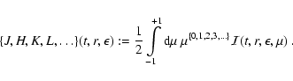
Momentum space is described by the coordinates
were suppressed for brevity.
Momentum space is described by the coordinates ![]() and
and ![]() ,
which are the energy and the cosine of the angle of propagation
of the neutrino with respect to the radial direction, both measured in
the locally comoving frame of reference.
Note that the opacity
,
which are the energy and the cosine of the angle of propagation
of the neutrino with respect to the radial direction, both measured in
the locally comoving frame of reference.
Note that the opacity ![]() and the emissivity
and the emissivity ![]() ,
and thus the
collision integral
,
and thus the
collision integral
![]() in general depend also
explicitly on momentum-space
integrals of
in general depend also
explicitly on momentum-space
integrals of ![]() ,
which makes the transfer equation an
integro-partial differential equation.
Examples of the actual computation of the collision integral for a
number of interaction processes of neutrinos with matter can
be found in Appendix A.
,
which makes the transfer equation an
integro-partial differential equation.
Examples of the actual computation of the collision integral for a
number of interaction processes of neutrinos with matter can
be found in Appendix A.
In general, the metric functions
![]() and
R(t,a) have to be computed numerically from the Einstein
field equations.
When working to order
and
R(t,a) have to be computed numerically from the Einstein
field equations.
When working to order
![]() and in a flat
spacetime (usually called the "Newtonian approximation''), it is
however possible to express these functions analytically in terms of
only the velocity field and its first time derivative (the fluid
acceleration).
Details of the derivation can be found in Castor (1972).
Alternatively one can simply reduce the special relativistic
transfer equation (Mihalas 1980) to order
and in a flat
spacetime (usually called the "Newtonian approximation''), it is
however possible to express these functions analytically in terms of
only the velocity field and its first time derivative (the fluid
acceleration).
Details of the derivation can be found in Castor (1972).
Alternatively one can simply reduce the special relativistic
transfer equation (Mihalas 1980) to order
![]() .
.
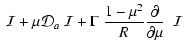
This transfer equation, together with its
angular moment equations of zeroth and first order reads
(e.g., Mihalas & Mihalas 1984, see also Lowrie et al. 2001):
 |
(9) |
For reference we also write down the transformations
(correct to
![]() )
which allow one to relate the
frequency-integrated moments in the
comoving ("Lagrangian'') and in the inertial ("Eulerian'') frame of
reference (indicated by the superscript "Eul'').
)
which allow one to relate the
frequency-integrated moments in the
comoving ("Lagrangian'') and in the inertial ("Eulerian'') frame of
reference (indicated by the superscript "Eul'').
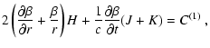
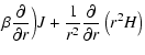
The system of Eqs. (6)-(8) is coupled to the
evolution equations of the
fluid (Eqs. (1)-(4)) in spherical
coordinates and symmetry) by virtue of the
definitions of the source terms
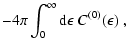
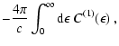
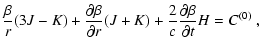
Recently, Lowrie et al. (2001) emphasized the fundamental significance
of a term
In core-collapse supernova simulations carried out so far, the dynamics of the stellar fluid presumably was not affected by neglecting the term in Eq. (6). However, our tests with Eq. (6), including the additional time derivative of Eq. (14) and the corresponding changes in the moment equations (Eqs. (7), (8)), have shown that the neutrino signal computed in a supernova simulation is indeed altered compared to the traditional treatment. We will therefore take the term of Eq. (14) into account in future simulations.
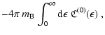
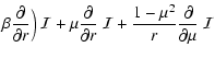
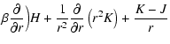
For calculating nonrelativistic problems
Mihalas & Mihalas (1984) suggested a form of the radiation momentum
equation (Eq. (8)), in which all velocity-dependent terms
except
for the
![]() -term in the first line of
Eq. (8) are dropped.
When the velocities become sizeable, however, it may be advisable
to solve the momentum equation in its general form
(Eq. (8)).
Doing so, we indeed found that the terms omitted by Mihalas & Mihalas (1984)
can have an effect on the solution of the neutrino transport in
supernovae, in particular on the neutrino energy spectrum.
-term in the first line of
Eq. (8) are dropped.
When the velocities become sizeable, however, it may be advisable
to solve the momentum equation in its general form
(Eq. (8)).
Doing so, we indeed found that the terms omitted by Mihalas & Mihalas (1984)
can have an effect on the solution of the neutrino transport in
supernovae, in particular on the neutrino energy spectrum.
Copyright ESO 2002
![$\displaystyle \frac{\partial}{\partial \mu}
\left[
\left(1-\mu^2\right)\left\{
...
...R}
-\frac{1}{c}{\cal D}_t\Lambda\Big)
-{\cal D}_a\Phi \right\}~{\cal I}
\right]$](/articles/aa/full/2002/46/aa2451/img78.gif)
![$\displaystyle \frac{\partial}{\partial \epsilon}
\left[
\epsilon~\Big(
\left(1-...
...}
+\mu^2\frac{1}{c}{\cal D}_t\Lambda
+\mu {\cal D}_a\Phi
\Big)~{\cal I}
\right]$](/articles/aa/full/2002/46/aa2451/img79.gif)
![$\displaystyle \frac{\partial}{\partial \mu}\left[(1-\mu^2)
\left\{\mu\Big(\frac...
...r}\Big)-\frac{1}{c}\frac{\partial \beta}{\partial t} \right\}~
{\cal I} \right]$](/articles/aa/full/2002/46/aa2451/img96.gif)
![$\displaystyle \frac{\partial}{\partial \epsilon}\left[\epsilon~\Big((1-\mu^2)
\...
...ial
r}+\mu \frac{1}{c}\frac{\partial \beta}{\partial t} \Big)
~{\cal I} \right]$](/articles/aa/full/2002/46/aa2451/img97.gif)
![$\displaystyle \frac{\partial}{\partial \epsilon}\left[\epsilon\left(\frac{\beta...
...eta}{\partial r}K+\frac{1}{c}\frac{\partial \beta}{\partial t}H
\right) \right]$](/articles/aa/full/2002/46/aa2451/img100.gif)
![$\displaystyle \frac{\partial}{\partial
\epsilon}\left[\epsilon~\left(\frac{\bet...
...eta}{\partial r}L+\frac{1}{c}\frac{\partial \beta}{\partial t}K
\right) \right]$](/articles/aa/full/2002/46/aa2451/img103.gif)