3 Numerical implementation

3.1 Overview of the basic numerical strategy

For solving the neutrino radiation hydrodynamics problem we employ the well-known "operator splitting''-approach, a popular method to make large problems computationally tractable by considering them as a combination of smaller subproblems. The coupled set of equations of radiation hydrodynamics (Eqs. (1)-(4), (6)-(8)) is split into a "hydrodynamics part'' and a "neutrino part'', which are solved independently in subsequent ("fractional'') steps. In the "hydrodynamics part'' (Sect. 3.2) a solution of the equations of hydrodynamics including the effects of gravity is computed without taking into account neutrino-matter interactions.

In what we call the "neutrino part'' (Sects. 3.3-3.4) the coupled system of equations describing the neutrino transport and the changes of the specific internal energy e and the electron fraction ${Y_{\rm e}}$ of the stellar fluid due to the emission and absorption of neutrinos are solved. The latter changes are given by the equations

  

$$\frac{\delta}{\delta t} e= -\frac{4\pi}{\rho}\int_{0}^{\infty} {\... ...\sum_{\nu\in\{{\nu_{\rm e}},{\bar\nu_{\rm e}},\dots\}} C^{(0)}_\nu(\epsilon) ~,$$ (15)

$$\frac{\delta}{\delta t} {Y_{\rm e}}= -\frac{4\pi m_{\rm B}}{\rho}... ...}_{\nu_{\rm e}}(\epsilon)- \frak{C}^{(0)}_{\bar\nu_{\rm e}}(\epsilon)\right) ~.$$ (16)

Here, the notation $\delta/\delta t$ indicates that the full problem as given, e.g., by Eq. (4), is split into the equations $\partial_t(\rho {Y_{\rm e}}) + r^{-2} \partial_r~(r^2\rho {Y_{\rm e}}~v) = 0$ and $\delta_t~{Y_{\rm e}}=Q_{\rm N}/\rho$.

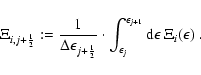
Within the neutrino part, we calculate in a first step the transport of energy and electron-type lepton number by neutrinos and the corresponding exchange with the stellar fluid for electron neutrinos ( ${\nu_{\rm e}}$) and antineutrinos ( ${\bar\nu_{\rm e}}$) only, which also means that the sum in Eq. (15) is restricted to $\nu \in \{{\nu_{\rm e}}, {\bar\nu_{\rm e}}\}$. The $\mu$ and $\tau$ neutrinos and their antiparticles, all represented by a single species ("${\nu_x}$'') are handled together with the remaining terms of the sum in Eq. (15) in a second step.

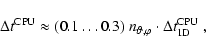
For the neutrino transport we use the so-called "variable Eddington factor'' method, which determines the neutrino phase-space distribution by iteratively solving the radiation moment equations for neutrino energy and momentum coupled to the Boltzmann transport equation. Closure of the set of moment equations is achieved by a variable Eddington factor calculated from a formal solution of the Boltzmann equation, and the integro-differential character of the latter is tamed by making use of the integral moments of the neutrino distribution as obtained from the moment equations. The method is similar to the one described by Burrows et al. (2000).

  
3.2 The hydrodynamics code

For the integration of the equations of hydrodynamics we employ the Newtonian finite-volume hydrodynamics code PROMETHEUS developed by Fryxell et al. (1989). PROMETHEUS is a direct Eulerian, time-explicit implementation of the Piecewise Parabolic Method (PPM) of Colella & Woodward (1984), which is a second-order Godunov scheme employing a Riemann solver. PROMETHEUS is particularly well suited for following discontinuities in the fluid flow like shocks or boundaries between layers of different chemical composition. It is capable of tackling multi-dimensional problems with high computational efficiency and numerical accuracy.

The version of PROMETHEUS used in our radiation hydrodynamics code was provided to us by Keil (1997). It offers an optional generalization of the Newtonian gravitational potential to include general relativistic corrections. The hydrodynamics code was considerably updated and augmented by K. Kifonidis who added a simplified version of the "Consistent Multifluid Advection (CMA)'' method (Plewa & Müller 1999) which ensures an accurate advection of the individual chemical components of the fluid. In order to avoid spurious oscillations arising in multidimensional simulations, when strong shocks are aligned with one of the coordinate lines (the so-called "odd-even decoupling'' phenomenon), a hybrid scheme was implemented (Kifonidis 2000; Plewa & Müller 2001) which, in the vicinity of such shocks, selectively switches from the original PPM method to the more diffusive HLLE solver of Einfeldt (1988).

  
3.3 Multi-group formulation of the $\mathsf{{\cal O}(v/c)}$ moment equations

In what follows we describe the numerical implementation of the "Newtonian'' limit of the transport equations including ${\cal O}(v/c)$-terms (cf. Sect. 2.2.2). The general relativistic version of the code is based on almost exactly the same considerations.

  
3.3.1 General considerations

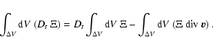
In order to construct a conservative numerical scheme for the system of moment equations, we integrate the moment equations (Eqs. (7), (8)) over a zone of the numerical $(r,\epsilon)$-mesh.

Spatial discretization:

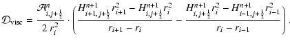
After having performed the integral over the volumes $\Delta V$ of the radial mesh zones, the moment equations can be rewritten as evolution equations for the volume-integrated moments (e.g.,  $\int_{\Delta V}J~{\rm d}V$). In case of a moving radial grid, where the volume $\Delta V$ of a grid cell is time dependent, one has to apply the "moving grid transport theorem'' (see e.g. Müller 1991) in order to interchange the operators D_t and $\int_{\Delta V}{\rm d}V$. For the special case of a Lagrangian grid, where the grid moves with the velocity of the stellar fluid, the latter reads:

$$\int_{\Delta V}{\rm d}V~(D_t~\Xi)= D_t\int_{\Delta V} {\rm d}V~ \Xi - \int_{\Delta V}{\rm d}V~(\Xi~ {\rm div}~ \vec{v}) ~.$$ (17)

Here and in the following the symbol $\Xi$ represents one of the moments J or H (and also ${\cal J}:=\epsilon^{-1}J$ or ${\cal H}:=\epsilon^{-1}H$).

The computational domain $r_{\rm min} \le r \le r_{\rm max}$ is covered by N_r radial zones. As the zone center $r_{i+{\frac{1}{2}}}$ we define the volume-weighted mean of the interface coordinates r_i and r_i+1:

$$r_{i+{\frac{1}{2}}}:=\left(\frac{1}{2}~\left(r_i^3+r_{i+1}^3\right)\right)^{1/3},\quad i=0,\dots,N_r-1 ~.$$ (18)

Scalar quantities like $J_{i+{\frac{1}{2}}}$, $K_{i+{\frac{1}{2}}}$ are defined on zone centers, whereas vectors like H_i and L_ilive on the interfaces of radial zones. "Miscentered'' values like, e.g,. J_i or $H_{i+{\frac{1}{2}}}$, are in general computed by linear interpolation, using the values of the nearest neighbouring coordinates ( $J_{i-{\frac{1}{2}}}$ and $J_{i+{\frac{1}{2}}}$, or H_i and H_i+1, respectively).

Spectral discretization:

The spectral range $0\le \epsilon \le \epsilon_{\rm max}$ is covered by a discrete energy grid consisting of $N_\epsilon$ energy "bins'', where the centers of these zones are given in terms of the interface values as

$$\epsilon_{j+{\frac{1}{2}}}:=\frac{1}{2}~(\epsilon_{j}+\epsilon_{j+1}),\quad j=0,\dots,N_\epsilon-1 ~,$$ (19)

and the width of an energy bin is denoted by ${\Delta\epsilon}_{j+{\frac{1}{2}}} :=\epsilon_{j+1}-\epsilon_{j}$. The radiation moments are interpreted as average values within energy bins:

$$\Xi_{i,j+{\frac{1}{2}}}:= \frac{1}{{\Delta \epsilon}_{j+{\fr... ...\epsilon_j}^{\epsilon_{j+1}}{\rm d}\epsilon~\Xi_i(\epsilon) ~.$$ (20)

Time differencing:

We employ a time-implicit finite differencing scheme for the moment equations (Eqs. (7), (8)) in combination with the equations which describe the exchange of internal energy and electron fraction with the stellar medium (Eqs. (15), (16)). Doing so we avoid the restrictive Courant Friedrichs Lewy (CFL) condition which explicit numerical schemes have to obey for stability reasons: for neutrino transport in the optically thin regime the CFL condition would require $c\Delta t < \Delta r$, where $\Delta r$ is the size of the smallest zone and $\Delta t$ the numerical time step. Even more importantly, the time-implicit discretization allows one to efficiently cope with the different time scales of the problem: the "stiff'' source terms introduce a characteristic time scale proportional to the mean free path $\lambda$ of the neutrinos, $c\Delta t = \lambda=\Delta r/\Delta\tau$, which can be orders of magnitude smaller than the CFL time step in the opaque interior of a protoneutron star, where the optical depth $\Delta\tau$ of individual grid cells becomes very large.

  
3.3.2 Finite differencing of the moment equations

Applying the procedures described in Sect. 3.3.1 to the moment equations (Eqs. (7), (8)) we obtain for each neutrino species $\nu\in\{{\nu_{\rm e}},{\bar\nu_{\rm e}},\nu_{\mu},\dots\}$ (the corresponding index is suppressed in the notation below) the finite differenced moment equations. On an Eulerian grid they read:

 

$$\frac{J_{i+{\frac{1}{2}},j+{\frac{1}{2}}}^{n+1}-J_{i+{\frac{1}{2}},j+{\frac{1}{2}}}^{n}} {ct^{n+1}-ct^{n}} \frac{4\pi}{\Delta V_{i+{\frac{1}{2}}}} \left(r_{i+1}^2H_{i+1,j+{\frac{1}{2}}}^{n+1}-r_{i}^2H_{i,j+{\frac{1}{2}}}^{n+1}\right)$$ +

$$\frac{4\pi}{\Delta V_{i+{\frac{1}{2}}}} \left(r_{i+1}^2\beta_{i+1... ...1}{2}}}- r_{i}^2\beta_{i}J_{\iota(i),j+{\frac{1}{2}}}^{ n+{\frac{1}{2}}}\right)$$ +

$$\frac{1}{{\Delta \epsilon}_{j+{\frac{1}{2}}}} \left\{ \epsilon_{j... ..._{i+{\frac{1}{2}},j+1} -\epsilon_j {[u\;J^{n+1}]}_{ i+{\frac{1}{2}},j} \right\}$$ -

$$\left[\frac{\beta}{r}\right]_{i+{\frac{1}{2}}}{[(1-f_K)\; J^{n+1}]}_{i+{\frac{1}{2}},j+{\frac{1}{2}}}$$ +

$$\left[\frac{\partial \beta}{\partial r}\right]_{ i+{\frac{1}{2}}}... ...{ i+{\frac{1}{2}},j+{\frac{1}{2}}}\; J_{ i+{\frac{1}{2}},j+{\frac{1}{2}}}^{n+1}$$ +

$$\frac{2}{c}\left[\frac{\partial \beta}{\partial t}\right]_{i+{\fr... ...{1}{2}},j+{\frac{1}{2}}} = {C^{(0)}}^{n+1}_{i+{\frac{1}{2}},j+{\frac{1}{2}}} ~,$$ + (21)

 

$$\frac{H_{i,j+{\frac{1}{2}}}^{n+1}-H_{i,j+{\frac{1}{2}}}^{n}} {ct^{n+1}-ct^{n}} \frac{4\pi}{\Delta V_{i}} (r_{i+{\frac{1}{2}}}^2{[f_K J^{n+1}]}_{... ...}{2}}}- r_{i-{\frac{1}{2}}}^2{[f_K J^{n+1}]}_{i-{\frac{1}{2}},j+{\frac{1}{2}}})$$ +

$$\frac{2\pi}{\Delta V_{i}}(r_{i+{\frac{1}{2}}}^2-r_{i-{\frac{1}{2}}}^2 )~ {[(f_K-1)~J^{n+1}]}_{i,j+{\frac{1}{2}}}$$ +

$$\frac{4\pi}{\Delta V_{i}}\left( r_{i+{\frac{1}{2}}}^2\beta_{i+{\f... ...rac{1}{2}}}H_{\iota(i-{\frac{1}{2}}),j+{\frac{1}{2}}}^{ n+{\frac{1}{2}}}\right)$$ +

$$\frac{1}{{\Delta \epsilon}_{j+{\frac{1}{2}}}} \left\{ \epsilon_{j+1} {[w\;J^{n+1}]}_{i,j+1} -\epsilon_j {[w\;J^{n+1}]}_{ i,j} \right\}$$ -

$$\left[\frac{\partial \beta}{\partial r}\right]_{i}\;H_{ i,j+{\fra... ...{f_K})\; J^{n+1}]}_{ i,j+{\frac{1}{2}}} ={C^{(1)}}^{n+1}_{i,j+{\frac{1}{2}}} ~.$$ + (22)

Note that by virtue of introducing the "Eddington factors'' (see the following section for their actual computation) f_H:=H/J, f_K:=K/J and f_L:=L/J, the system of moment equations has been closed. The "flux'' in energy space across the boundaries between energy zones appearing in the third and fifth line of Eq. (21) and Eq. (22), respectively, is given in terms of the interface values $J_{i+{\frac{1}{2}},j}$, which are defined as the geometrical mean of $J_{i+{\frac{1}{2}},j-{\frac{1}{2}}}$ and $J_{i+{\frac{1}{2}},j+{\frac{1}{2}}}$, and the advection velocities

 

$$u_{i+{\frac{1}{2}},j}:= \left[\frac{\beta}{r}\right]_{i+{\frac{1}... ...rtial \beta}{\partial t}\right]_{i+{\frac{1}{2}}} {[f_H]}_{i+{\frac{1}{2}},j}~,$$ (23)

 

$$w_{i,j}:= \left[\frac{\beta}{r}\right]_{i}{[f_H-f_L]}_{i,j} + \le... ... \frac{1}{c}\left[\frac{\partial \beta}{\partial t}\right]_{i} {[f_K]}_{i,j} ~.$$ (24)

The nonlinear interpolation of J in energy space turned out to be crucial for obtaining a numerically stable algorithm. The Eddington factors f_H, f_K and f_L are interpolated linearly in energy space in order to avoid problems in case the odd moments (H or L) change their signs.

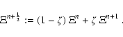
Since the radiation moments are defined on a staggered mesh, the finite-difference equations are second-order accurate in space. First-order accuracy in time is achieved by employing fully implicit time-differences ("backward Euler''). Only the advection terms in the second and forth line of Eq. (21) and Eq. (22), respectively, are treated differently (see Sect. 4.3.1 for a motivation):

$$\Xi^{n+{\frac{1}{2}}}:= (1-\zeta)~\Xi^{n}+\zeta~\Xi^{n+1} ~.$$ (25)

For stability reasons, the interpolation parameter $\zeta=0.51$ was chosen slightly larger than 0.5, which makes the treatment of the advection terms "almost'' second-order accurate in time (see, e.g. Dorfi 1998). The interface values $J_{\iota}$ and $H_{\iota}$ are taken as the corresponding upwind quantities with

$$\iota(i):= \left\{ \begin{array}{ll} i-\frac{1}{2}&\quad {\rm... ...[2mm] i+\frac{1}{2}&\quad {\rm else}~. \\ \end{array}\right.$$ (26)

In order to damp spurious oscillations behind sharp neutrino pulses travelling through nearly transparent zones, an additional diffusive term is added to the left-hand side of the first moment equation (Eq. (22)). Its finite-differenced form is (Blinnikov et al. 1998):

 

$${\cal D}_{\rm visc}=\frac{{\cal A}^n_{i,j+{\frac{1}{2}}}}{2~r_i^2... ...1}{2}}}r_{i}^2-H^{n+1}_{i-1,j+{\frac{1}{2}}}r_{i-1}^2}{r_{i}-r_{i-1}} \Bigg) ~.$$ (27)

In effect this term resembles the diffusivity of the donor cell scheme and hence allows one to selectively switch from the second order radial discretization to a first order scheme. Following Blinnikov et al. (1998) the (energy dependent) "artificial radiative viscosity'' ${\cal A}$ is set to unity in transparent zones and goes to zero for optical depth $\Delta \tau \gtrsim 1$. By construction the diffusive term vanishes when the luminosity H r² does not depend on radius and hence is only active during transient phases when sharp neutino pulses propagate across the grid.

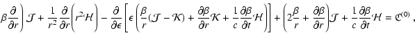
Using a similar diffusive term in the zeroth moment equation (Eq. (21)) allowed us also to overcome stability problems with the numerical handling of the velocity-dependent terms in the general form of the radiation momentum equation, Eq. (8).

  
3.3.3 Boundary conditions

For the solution of the moment equations (Eqs. (7), (8)), boundary conditions have to be specified at $r=r_{\rm min}$, $r=r_{\rm max}$, $\epsilon=0$ and $\epsilon=\epsilon_{\rm max}$. In the radial domain the values of quantities at the boundaries are iteratively obtained from the solution of the Boltzmann equation (see Sect. 3.4.3 for the boundary conditions employed there), which has the advantage that in the moment equations no assumptions have to be made about the angular distribution of the specific intensity at the boundaries. Specifically, at the inner boundary $H_{0,j+{\frac{1}{2}}}$ is given by $H(t,r=r_{\rm min},\epsilon)$ as computed from the Boltzmann equation. To handle the outer boundary, we apply Eq. (22) on the "half shell'' between $r_{N_r-{\frac{1}{2}}}$ and r_Nr (Mihalas & Mihalas 1984). Where necessary, $J_{N_r+{\frac{1}{2}},j+{\frac{1}{2}}}$ is replaced by $H_{N_r,j+{\frac{1}{2}}}/[{f_H}]_{N_r,j+{\frac{1}{2}}}$ in Eqs. ((21), (22)).

At $\epsilon=0$ the flux in energy space vanishes and hence we simply set $\epsilon_0 u_{i+{\frac{1}{2}},0}J_{ i+{\frac{1}{2}},0}^{n+1}=0$ in Eq. (21). At the upper boundary of the spectrum the flux in energy space, $\epsilon_{N_\epsilon} u_{i+{\frac{1}{2}},N_\epsilon}J_{i+{\frac{1}{2}},N_\epsilon}^{n+1}$ is computed by a (geometrical) extrapolation of the moments $J_{i+{\frac{1}{2}},N_\epsilon-\frac{3}{2}}$ and $J_{i+{\frac{1}{2}},N_\epsilon-\frac{1}{2}}$ and by a linear extrapolation of the advection velocity using $u_{i+{\frac{1}{2}},N_\epsilon-\frac{3}{2}}$ and $u_{i+{\frac{1}{2}},N_\epsilon-\frac{1}{2}}$. Analogous expressions are used for Eq. (22).

3.3.4 Finite differencing of the source term

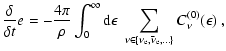
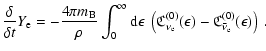
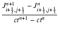
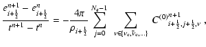
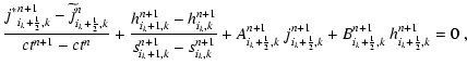
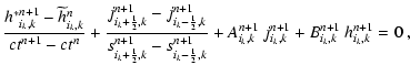
The finite differenced versions of the operator-splitted source terms in the energy and lepton number equations (Eqs. (15), (16)) of the stellar fluid read:

  

$$\frac{e_{i+{\frac{1}{2}}}^{n+1}-e_{i+{\frac{1}{2}}}^{n}} {t^{n+1}... ...\nu_{\rm e}},\dots\}}~ {C^{(0)}}^{n+1}_{i+{\frac{1}{2}},j+{\frac{1}{2}},\nu} ~,$$ (28)

$$\frac{{{Y_{\rm e}}}_{i+{\frac{1}{2}}}^{n+1}-{{Y_{\rm e}}}_{i+{\fr... ...k{C}^{(0)}}^{n+1}_{i+{\frac{1}{2}},j+{\frac{1}{2}},{\bar\nu_{\rm e}}} \right)~.$$ (29)

  
3.3.5 Neutrino number transport

In the finite-differenced version of the (monochromatic) neutrino energy equation (Eq. (21)) the derivative with respect to energy, $\partial/\partial\epsilon$, has been written in a conservative form. When a summation over all energy bins is performed in Eq. (21), the terms containing fluxes across the boundaries of the energy zones telescope and an appropriate finite differenced version of the total (i.e. spectrally integrated) neutrino energy equation is recovered. This essential property does, however, not hold automatically also for the neutrino number density ${\cal N}:= 4\pi/c ~ \int_0^\infty{\rm d}\epsilon~ {\cal J}(\epsilon)$, when the naive definition ${\cal J}_{i+{\frac{1}{2}},j+{\frac{1}{2}},\nu}:=J_{i+{\frac{1}{2}},j+{\frac{1}{2}},\nu}/\epsilon_{j+{\frac{1}{2}}}$is adopted. By inserting the latter expression into Eq. (21) and summing over all energy bins, it can easily be verified that the corresponding fluxes across the boundaries of the energy bins do not cancel anymore due to the finite cell size $\Delta\epsilon_{j+{\frac{1}{2}}}$.

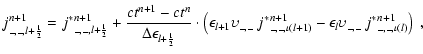
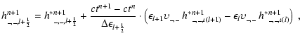
In order to avoid this problem, we instead derive the moment equations for ${\cal J}$ and ${\cal H}$ (by multiplying Eqs. (7), (8) with $\epsilon^{-1}$) and recast them into a conservative form:

 

$$\Bigg(\frac{1}{c}\frac{\partial}{{\partial t}} \beta\frac{\partial}{{\partial r}}\Bigg)~ {\cal J} + \frac{1}{r^2... ...cal J} +\frac{1}{c}\frac{\partial \beta}{\partial t}{\cal H} =\frak{C}^{(0)} ~,$$ + (30)

 

$$\Bigg(\frac{1}{c}\frac{\partial}{{\partial t}} \beta\frac{\partial}{{\partial r}}\Bigg)~ {\cal H} + \frac{1}{r^2... ...\right) +\frac{1}{c}\frac{\partial \beta}{\partial t}{\cal J} =\frak{C}^{(1)} .$$ + (31)

Equations (30), (31) are then discretized as a separate set of equations. Consequently, the finite-difference representation of the monochromatic number density ${\cal J}_{i+{\frac{1}{2}},j+{\frac{1}{2}}}$ and the monochromatic number flux ${\cal H}_{i,j+{\frac{1}{2}}}$ are now considered as new variables, which are determined by solving an extra set of two moment equations. Note that treating ${\cal J}_{i+{\frac{1}{2}},j+{\frac{1}{2}}}$ and ${\cal H}_{i,j+{\frac{1}{2}}}$ as additional variables is not necessarily in conflict with the relations ${\cal J}(\epsilon)\equiv J(\epsilon)/\epsilon$ and ${\cal H}(\epsilon)\equiv H(\epsilon)/\epsilon$ (${\cal K}$ and ${\cal L}$are defined likewise), which constitute dependences between the quantities. Since $J_{i+{\frac{1}{2}},j+{\frac{1}{2}}}$ and ${\cal J}_{i+{\frac{1}{2}},j+{\frac{1}{2}}}$, $H_{i,j+{\frac{1}{2}}}$ and ${\cal H}_{i,j+{\frac{1}{2}}}$ are defined as average values within the energy interval $[\epsilon_j,\epsilon_{j+1}]$ of different energy moments of the same function (rather than values of a function at point $\epsilon_{j+{\frac{1}{2}}}$; cf. Eq. (20)) they can be considered as variables that are independent of each other, provided that the inequalities $\epsilon_j \le \langle\epsilon\rangle_{i+{\frac{1}{2}},j+{\frac{1}{2}}} \le \epsilon_{j+1}$ with $\langle\epsilon\rangle_{i+{\frac{1}{2}},j+{\frac{1}{2}}} = J_{i+{\frac{1}{2}},j+{\frac{1}{2}}}/{\cal J}_{i+{\frac{1}{2}},j+{\frac{1}{2}}}$ or $\langle\epsilon\rangle_{i,j+{\frac{1}{2}}} = \vert H_{i,j+{\frac{1}{2}}}\vert/\vert{\cal H}_{i,j+{\frac{1}{2}}}\vert$are fulfilled (we thank our referee, A. Mezzacappa, for stressing the importance of this point). In practice, we find that this is always well fulfilled at high optical depths and low velocities. The constraint is violated only in the steeply falling, high-energy tail of the neutrino spectrum. Systematically inspecting results from simulations we find that a part of the spectrum is affected where $J_{i+{\frac{1}{2}},j+{\frac{1}{2}}}\Delta\epsilon_{i+{\frac{1}{2}},j+{\frac{1}{2}}}$ is less than one percent of the maximum value, which means that the energy integral over this spectral tail accounts for a negligible fraction of the total neutrino (energy) density.

3.3.6 Numerical solution

With the Eddington factors f_H, f_K, f_L and flow field $\beta$ being given, the nonlinear system of equations (Eqs. (21), (22), (30), (31), (28), (29)) is solved for the variables $\{J_{i+{\frac{1}{2}},j+{\frac{1}{2}}}, H_{i,j+{\frac{1}{2}}}, {\cal J}_{i+{\fr... ...1}{2}},j+{\frac{1}{2}}}, e_{i+{\frac{1}{2}}}, {{Y_{\rm e}}}_{i+{\frac{1}{2}}}\}$ by a Newton-Raphson iteration (e.g. Press et al. 1992), using the aforementioned boundary conditions.

This requires the inversion of a block-pentadiagonal system with 2 N_r+1 rows of blocks. The dimension of an individual block of the Jacobian is $(4N_\epsilon +2)$ in case of the transport of electron neutrinos and antineutrinos (the number of energy bins $N_\epsilon$ is multiplied by a factor of two because ${\nu_{\rm e}}$ and ${\bar\nu_{\rm e}}$ are treated as separate particles, the other factor of two comes from the additional transport of neutrino number). In contrast, muon and tau neutrinos and their antiparticles are considered here as one neutrino species because their interactions with supernova matter are roughly the same. In the absence of the corresponding charged leptons, muon and tau neutrinos are only produced (or annihilated) as $\nu\bar\nu$ pairs and hence do not transport lepton number. Therefore the blocks have a dimension of $(N_\epsilon +1)$ for these flavours.

For setting up the Jacobian all partial derivatives with respect to the radiation moments can be calculated analytically, whereas the derivatives with respect to electron fraction and specific internal energy are approximated by finite differences.

  
3.4 Formal solution of the Boltzmann equation

In order to provide the closure relations (the "variable Eddington factors'') for the truncated system of moment equations, we have to solve the Boltzmann equation. Since the emissivity $\eta$ and the opacity $\chi$ depend in general also on angular moments of ${\cal I}$, this is actually a nonlinear, integro-differential problem. However, $\eta$ and $\chi$ become known functions of only the coordinates t, r, $\epsilon$ and $\mu$, when J and H are used as given solutions of the moment equations. This allows one to calculate a formal solution of the Boltzmann equation.

3.4.1 Model equations

Making the change of variables (cf. Yorke 1980; Mihalas & Mihalas 1984; Körner 1992; Basheck et al. 1997)

$$(r,\mu)\mapsto(s:=\mu r,p:=r\sqrt{1-\mu^2}),\qquad\mu\ge 0 ~,$$ (32)

and introducing the symmetric and antisymmetric averages of the specific intensity

  

$$j(t,s,p):= \frac{1}{2}\big({\cal I}(\mu)+{\cal I}(-\mu)\big) ~,$$ (33)

$$h(t,s,p):= \frac{1}{2}\big({\cal I}(\mu)-{\cal I}(-\mu)\big) ~,$$ (34)

Eq. (6) can be split into two equations for j and h,

 

$$\frac{1}{c}\frac{{\rm D}}{{\rm D} t}j+ \frac{\partial}{\partial s... ...artial r}~j +\mu \frac{2}{c}\frac{\partial \beta}{\partial t}~ h = s_{\rm E} ~,$$ (35)

 

$$\frac{1}{c}\frac{{\rm D}}{{\rm D}t}h+ \frac{\partial}{\partial s}... ...r}\right) h +\mu \frac{1}{c}\frac{\partial \beta}{\partial t}~ j = u_{\rm E} ~.$$ (36)

The symmetric ($s_{\rm E}$) and antisymmetric ($u_{\rm E}$) averages of the source term C are defined in analogy to Eqs. (33), (34). Following Burrows et al. (2000, with our Eq. (38) correcting a misprint in their Eq. (24)) we have made the replacements

  

$$\left(\mu-\mu^3\right)\left(\frac{\partial \beta}{\partial r}-\frac{\beta}{r}\right)~\frac{\partial j}{\partial \mu} \to \left(3\mu^2-1\right)\left(\frac{\partial \beta}{\partial r}-\frac{\beta}{r}\right)~j ~,$$ (37)

$$\left(\mu-\mu^3\right)\left(\frac{\partial \beta}{\partial r}-\frac{\beta}{r}\right)~\frac{\partial h}{\partial \mu} \to \left(4\mu^2-2\right)\left(\frac{\partial \beta}{\partial r}-\frac{\beta}{r}\right)~h ~,$$ (38)

in deriving Eq. (35) and Eq. (36), respectively, from Eq. (6). This modification can be motivated as follows: As a consequence of Eqs. (37), (38) no more partial derivatives of the intensity (and hence j and h) with respect to $\mu$ appear in the model equations (Eqs. (35), (36)) of the original Boltzmann equation (Eq. (6)). This quality allows us to construct an efficient numerical solution scheme to be described in the next section. At the same time it is ensured that the monochromatic ${\cal O}(\beta)$moment equations (Eqs. (7), (8)) can be recovered when Eq. (35) and $\mu$ times Eq. (36) are integrated over angles. Thus, Eqs. (35), (36) are consistent with the monochromatic moment equations without including the exact aberration terms (see also Burrows et al. 2000). Moreover, the effects of angular aberration on the solution of the neutrino transport are found to be small (Liebendörfer, personal communication). Therefore we do not expect significant changes, in particular because only normalized moments H/J, K/J, L/J are computed from the solution of the Boltzmann equation to be used as closure relations in the moment equations.

  
3.4.2 Finite-difference equations

For the moment we shall ignore terms which contain frequency derivatives $\partial/\partial\epsilon$ (see Eqs. (35), (36)). These Doppler terms will be included in an operator-split manner.

Equations (35), (36) are then discretized on a so-called "tangent ray grid'' (for an illustration, see Fig. 1), the geometry of which being an immediate consequence of the transformation of variables given by Eq. (32). Applying this transformation, partial derivatives of only one momentum-space coordinate s remain, whereas the second coordinate p appears only in a parametric way (cf. Baschek et al. 1997). This greatly facilitates the numerical solution of the system.

Figure 1: Eulerian radial and tangent ray grid of the computation (solid lines) and virtual Lagrangian shell at time level $t^{n}=t^{n+1}-\Delta t$ (dotted). For simplicity we have assumed a radial motion of only one shell with index i. The filled circles mark the positions where j and h are known as the solutions of the previous time step on the Eulerian grid. For $v\not \equiv 0$ these positions do not coincide with the locations $(r_{i}^{\rm old},\mu _{ik}^{n+1})$, where initial values of the radiation field are required for computing the current time step (open circles). The latter positions are subject to the requirement that the ${\rm D}/{\rm D}t$ operator has to be evaluated at fixed radial Lagrangian and angular coordinates (The radial dashed lines connect points with constant angle cosines $\mu$ of tangent rays.).

A "tangent ray'' k is defined by its "impact parameter'' p_k=r_k at $\mu=0$. The coordinate s serves to measure the path length along the ray. On each tangent ray k, a staggered numerical mesh is introduced for the coordinate s. The zone boundaries (centers) of this mesh are given by the ray's intersections with the zone boundaries (centers) of the radial grid (cf. Fig. 1). With the "flux-like'' variable h being defined at the zone boundaries s_ik and the "density-like'' variable j being defined at the zone centers $s_{i+{\frac{1}{2}},k}$, the finite-differenced versions of Eqs. (35), (36) finally can be written down (cf. Mihalas & Klein 1982, Sect. V.2):

 

$$\frac{{j^*}^{n+1}_{i_k+{\frac{1}{2}},k}-\widetilde{j}^n_{i_k+{\fr... ...rac{1}{2}},k} +B_{i_k+{\frac{1}{2}},k}^{n+1}~h^{n+1}_{i_k+{\frac{1}{2}},k}=0 ~,$$ (39)

 

$$\frac{{h^*}^{n+1}_{i_k,k}-\widetilde{h}^n_{i_k,k}}{ct^{n+1}-ct^{n... ...}{2}},k}} +A_{i_k,k}^{n+1}~j^{n+1}_{i_k,k} +B_{i_k,k}^{n+1}~h^{n+1}_{i_k,k}=0~,$$ (40)

with the indices $k=K_0,\dots,N_r-1$ and $i_k=k,\dots,N_r-1$. If an inner boundary condition at some finite radius $r_{\rm min}>0$ is used, a number of "core rays'' $k=K_0,K_0+1,\dots,-1$ ( $-K_0\in {\rm I\!N}$), which penetrate the innermost radial shell ( $p_k \le r_{\rm min}$), can be defined in order to describe the angular distribution of the radiation at the inner boundary. For details, see e.g., Yorke (1980), Körner (1992), Dorfi (1998). The coefficients A and B are combinations of the velocity and angle-dependent terms and the source terms of Eqs. (35), (36). The definition of $\widetilde{j}$ and $\widetilde{h}$ will be given later, for the moment one may ignore the tilde symbol. We add a diffusive term to Eq. (40) analogous to the discussion in Sect. 3.3.2, replacing H r² in Eq. (27) by h.

The frequency derivatives of Eqs. (35), (36), which were ignored in the finite-difference versions, Eqs. (39), (40), are taken into account in a separate step by operator-splitting (the partially updated values for j and h were marked by asterisks in Eqs. (39), (40). The discretization of the corresponding terms is explicit in time and - provided the acceleration terms in the second line of Eqs. (35), (36) are neglected - can be performed straightforwardly using upwind differences in energy space ( $l=0,\dots,N_\epsilon-1$):

 

$$j^{n+1}_{\_,\_,l+{\frac{1}{2}}}={j^*}^{n+1}_{\_,\_,l+{\frac{1}{2}... ...a(l+1)} -\epsilon_{l} \upsilon_{\_,\_} ~{j^*}^{n+1}_{\_,\_,\iota(l)} \right) ~,$$ (41)

 

$$h^{n+1}_{\_,\_,l+{\frac{1}{2}}}={h^*}^{n+1}_{\_,\_,l+{\frac{1}{2}... ...a(l+1)} -\epsilon_{l} \upsilon_{\_,\_} ~{h^*}^{n+1}_{\_,\_,\iota(l)} \right) ~,$$ (42)

with

$$\iota(l):= \left\{ \begin{array}{ll} l-\frac{1}{2} &{\rm for... ...~, \\ [2mm] l+\frac{1}{2} &{\rm else}~, \\ \end{array}\right.$$ (43)

and

$$\upsilon_{i_k,k}:= (1-\mu_{i_k,k}^2)\left[\frac{\beta}{r}\rig... ...i_k,k}^2\left[\frac{\partial\beta}{\partial r}\right]_{i_k} ~,$$ (44)

where, for better readability, dashes replace the appropriate index pairs corresponding to radius and impact parameter, (i_k+1/2,k) in Eq. (41) and (i_k,k) in Eq. (42), respectively.

It should be possible to proceed along similar lines for including the exact aberration effects in the Boltzmann solution which, for the time being, includes aberration only in an approximate way on the basis of the replacements given by Eqs. (37), (38). In practice, however, the adopted tangent-ray geometry does not allow for a conservative discretization of the angular derivatives in a way as simple as in the case of the frequency derivatives. We plan to spend extra work on the omitted angular derivatives of the intensity in order to include them in future version of our code.

  
3.4.3 Boundary conditions

On the tangent ray grid boundary conditions must be specified for each ray k at s_k,k and at s_Nr,k. At the inner core radius ( $i=0;~ k=K_0,\dots, 0$ and $s_{-{\frac{1}{2}},k} :=s_{0,k}$) we set the boundary condition $j_{-{\frac{1}{2}},k}:={\cal I}^+_{0,k}-h_{0,k}$, with ${\cal I}^+_{0,k}:={\cal I}(t,r_{\rm min},\mu_{0,k})$. For the remaining rays ( $k=1,\dots, N_r$), symmetry and Eq. (34) imply h_k,k=0, since $\mu_{k,k}=0$.

At the outer radius ( $i=N_r;~ k=K_0,\dots,N_r$ and $s^{n+1}_{N_r+{\frac{1}{2}},k}:=s^{n+1}_{N_r,k}$) we consider Eq. (40) on the "half shell'' between $r_{N_r-{\frac{1}{2}}}$ and r_Nr (cf. Sect 3.3.3) and make the replacement $j_{N_r+{\frac{1}{2}},k}:={\cal I}^-_{N_r,k}+h_{N_r,k}$, with ${\cal I}^-_{N_r,k}:={\cal I}(t,r=r_{\rm max},-\mu_{N_r,k})$.

The physical boundary conditions are described by the functions ${\cal I}(t,r_{\rm min},\mu)$ and ${\cal I}(t,r_{\rm max},-\mu)$ with $0\le \mu \le 1$, which specify the specific intensity entering the computational volume at the inner and outer surfaces, respectively.

At the boundaries of the energy grid we use the same type of boundary conditions as described for the moment equations (cf. Sect. 3.3.3).

3.4.4 Numerical solution

By virtue of the approximations used to derive the model equations (Eqs. (35), (36)) and upon introducing the tangent ray grid, the system of Eqs. (39), (40) with suitably chosen boundary conditions can be solved independently for each impact parameter p_k, each type of neutrino (note that for simplicity we have dropped the index $\nu$ in our notation), and - because Doppler shift terms are split off - each neutrino energy bin $\epsilon_{j+{\frac{1}{2}}}$ (index also suppressed).

For the same reasons as detailed in Sect. 3.3, we have employed fully implicit ("backward Euler'') time differencing. Solving Eqs. (39), (40) therefore requires the separate solution of $N_k \times N_\epsilon \times N_\nu$ ( N_k:=N_r-K₀+1 is the number of tangent rays) pentadiagonal linear systems of dimension $\le$N_r. On vector computers, this can be done very efficiently by employing a vectorization over the index k. Once the numerical solution for j and h has been obtained, the monochromatic angular moments and thus the Eddington factors f_H=H/J, f_K=K/J and f_L=L/J can be computed using the numerical quadrature formulae

    

$$\int_0^1{\rm d}\mu~j(r_i,\mu)\approx \sum_{k=K_0}^{i} j_{ik} a_{ik} ~,$$ J(r_i) = (45)

$$\int_0^1{\rm d}\mu~\mu h(r_i,\mu)\approx \sum_{k=K_0}^{i} h_{ik} b_{ik} ~,$$ H(r_i) = (46)

$$\int_0^1{\rm d}\mu~\mu^2j(r_i,\mu)\approx \sum_{k=K_0}^{i} j_{ik} c_{ik} ~,$$ K(r_i) = (47)

$$\int_0^1{\rm d}\mu~\mu^3h(r_i,\mu)\approx \sum_{k=K_0}^{i} h_{ik} d_{ik} ~.$$ L(r_i) = (48)

Explicit expressions for the quadrature weights a_ik, b_ik and c_ik can be found in Yorke (1980), d_ik is calculated in analogy.

Unless the velocity field vanishes identically (in this case $\widetilde{j}\equiv j$ and $\widetilde{h}\equiv h$ in Eqs. (39) and (40), respectively), an additional complication arises, since the partial derivative ${\rm D}/{\rm D}t$ has to be evaluated not only at fixed Lagrangian radius (the index i in our case) but also for a fixed value of the angle cosine $\mu$. The angular grid $\{\mu_{ik}^n\}_{k=K_0\dots i}$, which is associated with the radius r_iⁿ, however, changes as r_i moves with time. As a consequence, e.g., the values of h at the old time level used in Eq. (40) are $\widetilde{h}^n_{ik}:=h(t^n,r_{i}^n,\mu_{ik}^{n+1})$ and not $h^n_{ik}:=h(t^n,r_{i}^n,\mu_{ik}^n)$, the solution of the previous time step (cf. Mihalas & Mihalas 1984, Sect. 98). At the beginning of the time step we therefore have to interpolate the radiation field for each fixed radial index i from the $\{\mu_{ik}^n\}_{k=K_0\dots i}$-grid onto the $\{\mu_{ik}^{n+1}\}_{k=K_0\dots i}$-grid. If an Eulerian grid is used for the computation, an additional interpolation in the radial direction is performed to map from the fixed r_i-grid to the coordinates given by $r_{i}^{\rm old}:=r_{i}-v_i\Delta t$ (see Fig. 1). This seemingly complicated procedure has the advantage of being computationally much more efficient than directly discretizing Eqs. (35), (36) in Eulerian coordinates. In this case the $v\partial_r$-term, which originates from making the replacement ${\rm D}_t=\partial_t+v\partial_r$, would couple grid points of different impact parameters and would therefore defy an independent treatment of the tangent rays.

3.5 Iteration procedure

A transport time step starts by adopting guess values (e.g., given by the solution of the previous time step) for J, H, ${Y_{\rm e}}$, and e. The quantities ${Y_{\rm e}}$, e and the density $\rho$ determine the thermodynamic state and thus the temperature and chemical potentials. These, together with J and H are used to evaluate the rhs of the Boltzmann equation. This allows one to compute its formal solution and the Eddington factors as detailed in Sect. 3.4. The Eddington factors are then fed into the system of moment and source-term equations, the solution of which (Sect. 3.3) yields improved values for J, H, ${Y_{\rm e}}$, and e. At this point, where required (e.g., for evaluating $\frak{C}^{(0)}$), the neutrino number density ${\cal J}$ and number flux density ${\cal H}$ are conventionally replaced by $\epsilon^{-1}J$ and $\epsilon^{-1}H$. This procedure is iterated until numerical convergence is achieved. With the Eddington factors being known from the described iteration procedure, the complete system of source-term and moment equations for neutrino energy and number is solved (once) in order to accomplish lepton number conservation. In this step ${\cal J}$ and ${\cal H}$ are treated as additional variables (cf. Sect. 3.3.5).

   
3.6 Details of coupling neutrino transport and hydrodynamics

Our experience with the operator-splitting technique has shown that considerable care is necessary in how precisely the equations of hydrodynamics are coupled with the neutrino transport and how the fractional time steps are scheduled. In the following we therefore describe the used procedures in some detail.

Since the hydrodynamics code and the transport solver in general have different requirements for numerical resolution, accuracy and stability, the discretization in both space and time of the two code components is preferably chosen to be independent of each other. In supernova simulations, for example, the time step limit (from the CFL condition) for the hydrodynamic evolution computed by a time-explicit method is typically more restrictive than in the time-implicit treatment of the transport part. Since the transport is computationally much more expensive, one wants to use a larger time step than for the hydrodynamics part. This means that a transport time step is divided into a suitable number of hydrodynamical substeps.

  
3.6.1 Schedule of updates

Starting from the hydrodynamic state $(\rho^n,e^n,{Y_{\rm e}}^n,v^n)$ at the old time level tⁿ, the time-explicit PPM algorithm first computes a solution of the hydrodynamical conservation laws without the effects of gravity and neutrinos. From the updated density, the gravitational potential can be calculated by virtue of Poisson's equation and finally the gravitational source terms are applied to the total energy equation (Eq. (3)) and the momentum equation (Eq. (2)). This completes the "hydrodynamics'' time step with size $\Delta t_{\rm Hyd}$, which is limited by the CFL-condition (see e.g., LeVeque 1992). By performing a total of $N_{\rm Hyd}^n$ substeps the hydrodynamic state is evolved from the time level tⁿ to the new time level tⁿ⁺¹ given by

$$t^{n+1}= t^n+\Delta t^n= t^n+\sum_{i=1}^{N_{\rm Hyd}^n}\Delta t^{i}_{\rm Hyd} ~,$$ (49)

where $N_{\rm Hyd}^n\in{\rm I\!N}$ is determined by the condition $\Delta t^n \le \Delta t^{\rm max}_{\rm Tr}$. Here $\Delta t^{\rm max}_{\rm Tr}$ is the maximum size for the transport time step, which is compatible with the constraints that the relative changes are at most 10% for the monochromatic neutrino energy and number density, and the relative changes of the density, temperature, internal energy density and electron fraction must not exceed values of a few percent during the time interval $\Delta t^n$. This leads to a partially updated hydrodynamic state $(\rho^{n+1},e^*,{Y_{\rm e}}^*,v^{*})$ which includes the effects due to hydrodynamic fluid motions and the acceleration by gravitational forces and neutrino pressure (see below). The corresponding state variables are then mapped onto the transport grid. During the transport time step of size $\Delta t^n$, the transport equations in combination with the evolution equations for the electron fraction and internal energy of the stellar medium in response to neutrino absorption and emission (Eqs. (28), (29)) are solved. This yields the source terms for energy and lepton number as $Q_{\rm E}=\rho^{n+1}\cdot (e^{n+1}-e^{*})/\Delta t^n$ and $Q_{\rm N}=\rho^{n+1}\cdot ({Y_{\rm e}}^{n+1}-{Y_{\rm e}}^{*})/\Delta t^n$. Since the transport grid in general does not necessarily coincide with the hydrodynamics grid, the new specific internal energy eⁿ⁺¹ and electron fraction ${Y_{\rm e}}^{n+1}$ as computed on the transport grid do not directly describe the new hydrodynamic state. Instead of interpolating the quantities eⁿ⁺¹ and ${Y_{\rm e}}^{n+1}$ back onto the hydrodynamics grid, we map the source terms by a conservative procedure and then update the electron number density and the total energy density on the hydrodynamics grid according to

  

$$[\rho \varepsilon]^{n+1}= \rho^{n+1}\varepsilon^{*}+ (Q_{\rm E}^{n+1}+v^{n+1}Q_{\rm M}^{n+1})\cdot\Delta t^n ~,$$ (50)

$$\rule{0pt}{0pt} [\rho {Y_{\rm e}}]^{n+1}= \rho^{n+1} {Y_{\rm e}}^*+ Q^{n+1}_{\rm N}\cdot\Delta t^n~.$$ (51)

Equations (50) and (51) express the effective influence of the source terms $Q_{\rm E}+vQ_{\rm M}$ and $Q_{\rm N}$ over the time of a transport step, but in fact we apply the corresponding sources (as given at the old time level) during each substep of the hydrodynamics. The quantities $\varepsilon^{*}$ and ${Y_{\rm e}}^*$ as needed for the transport part of the code, are recovered a posteriori by subtracting the accumulated effects of the neutrino sources again. The momentum equation of the stellar fluid is treated in a similar way. Accounting for the momentum transfer (acceleration) by neutrinos after each individual hydrodynamical substep (by using the old momentum source term $Q^n_{\rm M}$), however, is of crucial importance here. When a sizeable contribution of the neutrino pressure is ignored during a larger number of hydrodynamical substeps a potentially hydrostatic configuration can be severely driven out of mechanical equilibrium. Correspondingly, the fluid velocity v^* used in the transport step includes the effects due to the acceleration by neutrinos.

After the transport time step has been completed, the new neutrino stress $Q_{\rm M}^{n+1}$ is used for correcting v^* to give the new velocity vⁿ⁺¹ at time level tⁿ⁺¹:

$$[\rho v]^{n+1}=\rho^{n+1} v^{*}+ (Q_{\rm M}^{n+1}- Q_{\rm M}^{n}) \cdot \Delta t^n ~.$$ (52)

  
3.6.2 Arrangement of spatial grids

Radial discretization of the transport and hydrodynamic equations is done on independent grids. Therefore there is freedom to choose the number of zones and their coordinate values separately in both parts of the code. Only quantities which obey conservation laws have to be communicated from the hydro to the transport grid. By invoking the equation of state all other thermodynamical quantities can be derived from the density, the total energy density, momentum density and the number densities of electrons and nuclear species. In the other direction it is the neutrino source terms which have to be mapped back onto the hydro grid.

For the mapping procedure we assume the conserved quantities to be piecewise linear functions of the radius inside the grid cells, with parameters determined by the cell average values and so-called "monotonized slopes'' (for details see, e.g., Ruffert 1992 and references cited therein). In order to achieve global conservation of integral values we then simply average this function within each cell of the target grid of the mapping (cf. Dai & Woodward 1996).

Using this procedure in dynamical supernova simulations, we discovered spurious radial and temporal fluctuations of the temperature, electron fraction, entropy and related quantities inside the opaque protoneutron star unless the hydro and transport grids coincide exactly in this region. The scale of these fluctuations is sensitive to the radial cell size and the size of a time step, the relative amplitude was found to be typically of the order of a few percent, with the exact number varying between different quantities (see Rampp & Janka 2000). These fluctuations are understood from the fact that the mapping of the source terms on the one hand and the internal energy density (resp. temperature) on the other hand implies deviations from local thermodynamical equilibrium between neutrinos and stellar medium. The attempt of the neutrino transport to restore this equilibrium within a given grid cell leads to large net production or absorption rates, driving the temperature in the opposite direction and causing it to perform oscillations in time around a mean value. Despite these oscillations and fluctuations, the use of different numerical grids inside the protoneutron star did not cause noticeable problems for the accuracy of the "global'' evolution of our models, because the conservative mapping describes the exchange of energy and lepton number between neutrinos and the stellar fluid correctly on average.

Being cautious, we take advantage of the option of using different hydro and transport grids only during the early phases of the collapse and in regions of the star, where neutrinos are far from reaching equilibrium with the stellar fluid. In this case no visible fluctuations occur.

3.6.3 Conservation of total energy and lepton number

The numerical treatment of the radiation hydrodynamics problem should guarantee that the conservation laws for energy and lepton number are fulfilled.

Provided the acceleration terms ( $\propto\partial\beta/\partial t$), which are of order (v²/c²)and thus usually very small compared to the other terms, are ignored, the constancy of the total lepton number is ensured by, (a) a conservative discretization of the neutrino number equation (Eq. (30)), (b) a conservative handling of the electron number equation (Eq. (4)), and (c) the exact numerical balance of the source terms (cf. Eq. (13)) $-4\pi~ m_{\rm B}\int{\rm d}V~\int_0^\infty{\rm d}\epsilon~\frak{C}^{(0)}(\epsilon)$(defined on the transport grid) and $\int{\rm d}V~Q_{\rm N}$ (defined on the hydro grid). Point (a) requires that in Eq. (30) the flux divergence is discretized in analogy to the second line in Eq. (21) and that the $\beta~\partial{\cal J}/\partial r$ and $(2\beta/r+\partial\beta/\partial r)~{\cal J}$ terms are combined to ${\rm div} (\beta~{\cal J})$ to be discretized in analogy to the third line in Eq. (21). The energy derivative in Eq. (30) is treated in a conservative way as described in Sect. (3.3.5). Point (b) is achieved by the use of a conservative numerical integration of the electron number equation (Eq. (4)) in the spirit of the PROMETHEUS code, and requirement (c) is fulfilled by employing a conservative procedure for mapping the electron number source term from the transport grid to the hydro grid (see Sects. 3.6.1, 3.6.2). Doing so, the total lepton number remains constant in principle at the level of machine accuracy.

Different from the number transport, where the zeroth order moment equation for neutrinos by itself defines a conservation law, the derivation of a conservation law for the total energy implies a combination of the radiation energy and momentum equations. The use of a staggered radial mesh for discretizing the latter equations defies a suitable contraction of terms in analogy to the analytic case. Therefore our numerical description does not conserve neutrino energy with the same accuracy as neutrino number and the quality of total energy conservation has to be verified empirically for a given problem and numerical resolution.

For our supernova simulations, tests showed that neutrino number is conserved to an accuracy of better than 10^-11 per time step, while for neutrino energy a value below 10^-7 is achieved. With a typical number of about 50 000 transport time steps for a supernova simulation we thus find an empirical upper limit for the violation of energy conservation of $0.5\%$ of the neutrino energy. This translates to $0.05\%$ of the internal energy of the collapsed stellar core, i.e. a few times $10^{49}~{\rm erg}$ in absolute number. Errors of the same magnitude are introduced by the non-conservative treatment of the gravitational potential as a source term in the fluid-energy equation (Eq. (3)). Note that the use of different grids for the hydrodynamics and the transport does not affect the energy budget because we employ a conservative mapping of the neutrino source term between the grids (see Sects. 3.6.1, 3.6.2).

  
3.7 Approximate general relativistic treatment

We have not yet coupled our general relativistic version of the neutrino transport to a general relativistic hydrodynamics code. For the time being we work with a basically Newtonian code, which was extended to include post-Newtonian corrections of the gravitational potential. We hope that the deeper gravitational potential can account for the main effects of general relativity on stellar core collapse and the formation of neutron stars which do not approach gravitational instability to become black holes (cf. Bruenn et al. 2001). Because the general relativistic changes of the space-time metric are ignored, a consistent description of the neutrino transport requires that the fully relativistic equations are simplified such that only the effects of gravitational redshift and time dilation are retained.

3.7.1 Modified gravitational potential

By comparing the Tolman-Oppenheimer-Volkoff equation for hydrostatic equilibrium in general relativity (see, e.g., Kippenhahn & Weigert 1990, Sect. 2.6) with its Newtonian counterpart (cf. Eq. (2)) one can define a modified "gravitational potential'' which includes correction terms due to pressure and energy of the stellar medium and the neutrinos:

 

$$\Phi^{\rm GR}(r)= G \int\limits_\infty^r{\rm d}r'~ \frac{1}{{r'}^... ...\right) \frac{1}{\Gamma^2} \left(\frac{\rho_{\rm tot}c^2+p}{\rho c^2}\right) ~,$$ (53)

where $\rho_{\rm tot}c^2:=\rho (c^2 + e)$ is the total ("relativistic'') energy density and $P=4\pi/c\int_0^\infty {\rm d}\epsilon~ K$ the neutrino pressure. The calculation of the gravitational mass $m(r):=\int_0^r{\rm d}r'~4\pi {r'}^2(\rho_{\rm tot}+c^{-2}E+c^{-3}U F/\Gamma)$ takes into account contributions of neutrino energy density $E=4\pi/c\int_0^\infty {\rm d}\epsilon~ J$ and flux $F=4\pi\int_0^\infty {\rm d}\epsilon~ H$. The metric function $\Gamma$ is calculated as $\Gamma(r)=\sqrt{1+U(r)^2-2Gm(r)/rc^2}$ with the term U² accounting for the effects of fluid motion.

Equation (53) can be used in the Newtonian hydrodynamic equations (Eqs. (2), (3)) in order to approximately take into account general relativistic effects (cf. Keil 1997). The quality of this approach has to be ascertained empirically by comparison with fully general relativistic calculations. In our case such a comparison yields quite satisfactory results (see Sect. 4.3).

3.7.2 Approximate GR transport

The general relativistic moment equations describing transport of neutrino energy, momentum and neutrino number can be derived from the Lindquist-equation (cf. Eq. (5), Sect. 2.2.1). They are:

 

$$\frac{1}{c}\frac{{\rm D}}{{\rm D}t}~ J \frac{\Gamma}{R^2} \frac{\partial}{\partial R}(R^2H{\rm e}^{\Phi}) + \Gamma \partial_R {\rm e}^{\Phi}~ H$$ +

$$\frac{\partial}{\partial \epsilon}\left[ \epsilon~\Big( {\rm e}^{... ...+c^{-1} {\rm D}_t \Lambda~ K +\Gamma \partial_R {\rm e}^{\Phi}~ H \Big) \right]$$ -

$${\rm e}^{\Phi}\frac{U}{R}~(3J-K) +c^{-1}{\rm D}_t \Lambda~(J + K) ={\rm e}^{\Phi}~C^{(0)} ~,$$ + (54)

 

$$\frac{1}{c}\frac{{\rm D}}{{\rm D}t}~ H \frac{\Gamma}{R^2}\frac{\partial}{\partial R}(R^2K{\rm e}^{\Phi}) + \Gamma\partial_R {\rm e}^{\Phi}~ J +{\rm e}^{\Phi}\Gamma~\frac{K-J}{R}$$ +

$$\frac{\partial}{\partial \epsilon}\left[ \epsilon~\Big( {\rm e}^{... ...+c^{-1} {\rm D}_t \Lambda~ L +\Gamma \partial_R {\rm e}^{\Phi}~ K \Big) \right]$$ -

$$2({\rm e}^{\Phi}\frac{U}{R} +c^{-1}{\rm D}_t \Lambda)~H = {\rm e}^{\Phi}~C^{(1)} ~,$$ + (55)

for the energy transport, and

 

$$\frac{1}{c}\frac{{\rm D}}{{\rm D}t}~ {\cal J} \frac{\Gamma}{R^2} \frac{\partial}{\partial R}(R^2{\cal H}{\rm e}^{\Phi})$$ +

$$\frac{\partial}{\partial \epsilon}\left[ \epsilon~\Big( {\rm e}^{... ...D}_t \Lambda~ {\cal K} +\Gamma\partial_R {\rm e}^{\Phi}~ {\cal H} \Big) \right]$$ -

$$(2~{\rm e}^{\Phi}\frac{U}{R}+c^{-1}{\rm D}_t \Lambda)~{\cal J} ={\rm e}^{\Phi}~\frak{C}^{(0)} ~,$$ + (56)

 

$$\frac{1}{c}\frac{{\rm D}}{{\rm D}t}~ {\cal H} \frac{\Gamma}{R^2}\frac{\partial}{\partial R}(R^2{\cal K}{\rm e}^... ...rac{{\cal K}-{\cal J}}{R} +\Gamma \partial_R {\rm e}^{\Phi}~({\cal J}-{\cal K})$$ +

$$\frac{\partial}{\partial \epsilon}\left[ \epsilon~\Big( {\rm e}^{... ...}_t \Lambda~ {\cal L} +\Gamma \partial_R {\rm e}^{\Phi}~ {\cal K} \Big) \right]$$ -

$${\rm e}^{\Phi}\frac{U}{R}~({\cal H}+{\cal L}) + c^{-1} {\rm D}_t \Lambda~(2{\cal H}-{\cal L}) = {\rm e}^{\Phi}~\frak{C}^{(1)} ~,$$ + (57)

for the number transport.

In the approximate treatment we neglect the distinction between coordinate radius and proper radius ( $\partial_R \to \partial_r$, $\Gamma=1$) in Eqs. (54)-(57), and identify corresponding quantities with their Newtonian counterparts ($R\to r$, ${\rm e}^{\Phi}~U\to\beta$, $c^{-1}{\rm D}_t\Lambda \to \partial \beta/\partial r$). The same approximations are made in the "parent'' Boltzmann equation from which the moment equations of the relativistic approximation can be consistently derived. Accordingly, the approximations to Eqs. (54)-(57) contain only general relativistic redshift and time dilation effects for neutrinos. Coupling the transport with the Newtonian equations of hydrodynamics, these restrictions to a fully relativistic treatment are necessary in order to verify conservation laws for energy and lepton number of the coupled system.

Finite-difference versions of the moment equations and the corresponding parent Boltzmann equation for the approximate GR transport are obtained by applying the techniques described in Sects. 3.3 and 3.4. The lapse function is calculated by integrating the general relativistic Euler equation $\partial \ln~ {\rm e}^{\Phi}/\partial r=-(\rho_{\rm tot}c^2+p)^{-1}~(\partial p/\partial r-Q_{\rm M}/\Gamma)$ inward from the surface, where the boundary condition ${\rm e}^{\Phi}=\Gamma$ is applied (van Riper 1979).

  
3.8 Approximate multi-dimensional neutrino transport

Multi-dimensional frequency dependent neutrino transport in moving media and relativistic environments is a challenging problem for future work. Since convective phenomena were recognized to be highly important in supernovae (Herant et al. 1994; Burrows et al. 1995; Janka & Müller 1996; Keil et al. 1996 and refs. therein) one would of course like to perform simulations with Boltzmann neutrino transport also in two and three dimensions. Here we suggest an approximate approach based on a straightforward generalization of our variable Eddington factor method, which offers some advantages concerning computational efficiency. The approximation should be considered as an intermediate step between spherically symmetric and fully multi-dimensional models. Of course, the quality of the approximation for the neutrino transport which we will describe below, will finally have to be checked by a comparison with fully multi-dimensional transport calculations.

3.8.1 Basic considerations

Our approximate treatment may be a reasonably accurate and physically justifyable approach for describing neutrino transport in situations where the star does not show a global deformation (e.g., due to rotation) in layers which are opaque to neutrinos, but where inhomogeneities and anisotropies are present only on smaller scales (e.g., due to convection). Multi-dimensional hydrodynamical simulations suggest that convective processes occur in two distinct regions of the supernova core:

(a)

Convection inside the opaque protoneutron star causes deviations of the structural and thermodynamical quantities (like density or temperature) from spherical symmetry typically of the order of a few percent (Keil et al. 1996; Keil 1997). Moreover, the time scale for changes of such local fluctuations is short compared to the neutrino diffusion time scale. Hence, on the neutrino diffusion time scale no persistent local gradients in lateral and azimuthal directions are present in the dense stellar interior. This allows one to disregard the neutrino transport in these directions in a first approximation, which is at least correct in the temporal average.

(b)

Convective overturn motions occur between the neutrinospheres and the stalled hydrodynamic shock. Deviations from spherical symmetry are present there on larger angular scales (Herant et al. 1992; Herant et al. 1994; Burrows et al. 1995; Janka & Müller 1996; Müller & Janka 1997; Mezzacappa et al. 1998b; Kifonidis et al. 2000), but the neutrinos are only loosely coupled to the stellar medium in these regions. Therefore neutrino transport in the lateral directions does not play an important role and cannot have a significant influence on the local emission and absorption of neutrinos.

3.8.2 "Ray-by-ray'' transport

Under these circumstances the specific intensity ${\cal I}(t,r,\vartheta,\varphi, \epsilon,\vec{n})$can be assumed to depend mainly on r but only weakly on longitude $\varphi$ and latitude $\vartheta$ of the background medium. Hence, like in the spherically symmetric case, the dependence of the specific intensity on the direction of propagation $\vec{n}$ can be described by only one angle $\mu:=\vec{n}\cdot\vec{r}/\vert\vec{r}\vert$. The flux is thus approximated as $\vec{F}=4\pi\vec{r}/\vert\vec{r}\vert\cdot H(t,r,\vartheta,\varphi, \epsilon)$ and the scalar $P=4\pi/c\cdot K(t,r,\vartheta,\varphi, \epsilon)$ is sufficient to define the radiation stress tensor.

In the moment equations, gradients in the $\vartheta$- and the $\varphi$-direction, which describe the transport of energy and neutrino number into these lateral and azimuthal directions, are neglected, yet the parametric dependence of the (scalar) moments on the coordinates $\vartheta$ and $\varphi$ is retained and the radial transport is computed using the moment equations independently in each angular zone of the stellar model. In order to close the set of moment equations, variable Eddington factors are computed by iterating the Boltzmann equation and the corresponding moment equations on a spherically symmetric "image'' of the stellar background. The latter is defined as the angular average of physical quantities $\xi\in\{\rho,T,{Y_{\rm e}},\beta,\dots\}$ according to $\xi(t,r):=(4\pi)^{-1}\int_{-1}^{+1}{\rm d}\cos \vartheta~\int_{0}^{2\pi}{\rm d}\varphi~\xi(t,r,\vartheta,\varphi)$. Note that the variable Eddington factors are normalized moments of the neutrino phase space distribution function and thus should not show significant variation with the angular coordinates of the star. This justifies replacing them by quantities that depend only on the radial position and time.

Since for each latitude $\vartheta$ and longitude $\varphi$ the moment equations (Eqs. (7), (8)) in our approach are solved together with the evolution equations of electron fraction and internal energy due to neutrino sources (Eqs. (15), (16), local radiative equilibrium can be attained properly and conservation of energy can be fulfilled. It is not obvious to us how these fundamental requirements could be met in a more simple approximation where one uses a one-dimensional transport scheme to compute the transport on a spherically symmetric "mean star'', which is obtained at each time step by averaging the multi-dimensional hydrodynamical stellar model over angles.

3.8.3 Computational efficiency

Besides having significant advantages for easy and efficient implementation on vector and parallel computer architectures, the suggested approach also saves computer time compared to a multiple application of a one-dimensional Boltzmann solver. Let $\Delta t^{\rm CPU}_{1{\rm D}}$ be the computation time required for calculating a time step of the full one-dimensional transport problem and let $n^{\rm It}\in {\rm I\!N}$ be the number of steps that are necessary for the iteration between the moment equations and the Boltzmann equation to achieve convergence. If $n_{\vartheta,\varphi}:=n_{\vartheta}\cdot n_{\varphi}$ is the total number of angular zones that discretize the background star, the computation time for calculating one time step of the multi-dimensional problem with the described approximate method is

$$\Delta t^{\rm CPU}= \left(1+\frac{n_{\vartheta,\varphi}}{n^{\rm It}}\right)\cdot \Delta t^{\rm CPU}_{1{\rm D}} ~.$$ (58)

Note that the iteration procedure ( $n^{\rm It}> 1$) has to be performed only once, namely for calculating the Eddington factors on the angularly averaged "image'' of the background medium. With typical values of $n^{\rm It}=3\dots 10$ and large values of $n_{\vartheta,\varphi}$($\simeq$100) the computational effort for solving the multi-dimensional problem becomes about

$$\Delta t^{\rm CPU}\approx (0.1\dots 0.3)~ n_{\vartheta,\varphi}\cdot \Delta t^{\rm CPU}_{1{\rm D}} ~,$$ (59)

to be compared with $\Delta t^{\rm CPU}= n_{\vartheta,\varphi}\cdot \Delta t^{\rm CPU}_{1{\rm D}}$, which would be necessary for a straightforward multiple application of the one-dimensional method to a number of $n_{\vartheta,\varphi}$ angular zones.