

Up: Stellar evolution with rotation
We need now to express the quantity
 appearing in the previous sections.
According to the definition, one has
appearing in the previous sections.
According to the definition, one has
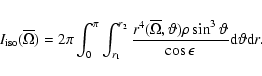
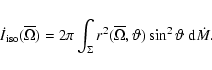
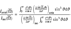
![$\displaystyle \dot{\mathcal{L}}_{{\rm excess}} = \left[ ~ \dot{I}_{{\rm anis}}(...
...anis}}(\overline{\Omega})}{\dot{I}_{{\rm iso}}(\overline{\Omega})} - 1\right] ,$](/articles/aa/full/2002/35/aa2544/img70.gif) |
|
|
(20) |
where
 and
and
 are the time variations
(negative values)
of the momentum of inertia due to the mass loss by
isotropic and anisotropic stellar winds respectively.
The momentum of
inertia
are the time variations
(negative values)
of the momentum of inertia due to the mass loss by
isotropic and anisotropic stellar winds respectively.
The momentum of
inertia
 in a shell between the
radii r1 and r2 in a star rotating
with angular velocity
in a shell between the
radii r1 and r2 in a star rotating
with angular velocity
 is
is
 |
(21) |
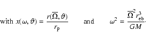
For a thin spherical shell of radius R and mass  ,
,
 is just the usual expression
 |
(22) |
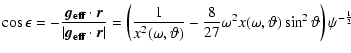
In a rotating star, the radial direction does not in
general coincide with the normal
to the surface (direction of the gravity). The angle  between the radial direction and the direction of the effective gravity
is a function of
between the radial direction and the direction of the effective gravity
is a function of
 and
and  ,
it is given by
,
it is given by
 |
|
|
(23) |
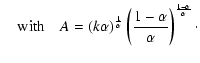
with
 |
|
|
(24) |
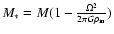
The effective gravity
 includes the effect
of the gravitational potential and centrifugal force, but
not the effect of radiation pressure (cf. Maeder & Meynet
2000). The rotation parameter
includes the effect
of the gravitational potential and centrifugal force, but
not the effect of radiation pressure (cf. Maeder & Meynet
2000). The rotation parameter  is the fraction of the angular break-up velocity.
The quantity
is the fraction of the angular break-up velocity.
The quantity
 is the ratio
of the radius at colatitude
with respect to the polar
radius
is the ratio
of the radius at colatitude
with respect to the polar
radius
 at break-up velocity. (Remark:
the exact value of the polar radius
at break-up velocity. (Remark:
the exact value of the polar radius
 also slightly depends on rotation through the structural
equations; this effect is accounted for in the numerical models.) The value of
is a solution of the equation of the stellar surface
in the Roche approximation
for given values of
and colatitude ,
i.e.
also slightly depends on rotation through the structural
equations; this effect is accounted for in the numerical models.) The value of
is a solution of the equation of the stellar surface
in the Roche approximation
for given values of
and colatitude ,
i.e.
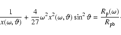 |
(25) |
 |
(26) |
 is the equatorial radius at break-up.
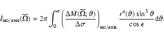
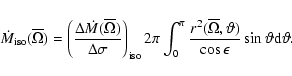
The time variation of the momentum of inertia by a star
which loses mass at a rate
is the equatorial radius at break-up.
The time variation of the momentum of inertia by a star
which loses mass at a rate  over its actual surface
 is
is
 |
(27) |
The quantity d
is defined by the local mass flux.
Usually an isotropic mass flux is considered in the stellar wind theory. However, for the reasons expressed in
Sect. 1, the mass loss in a rotating star is anisotropic.
Depending on whether we
consider the isotropic or anisotropic cases, we have
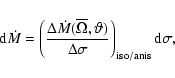 |
(28) |
where d refers to the surface element on the rotating star.
Thus, the corresponding expression for the time
variation of the momentum of inertia is in the isotropic
or anisotropic case
refers to the surface element on the rotating star.
Thus, the corresponding expression for the time
variation of the momentum of inertia is in the isotropic
or anisotropic case
 |
(29) |
The expression for the anisotropic mass flux has been obtained by the
application of the stellar wind theory to a rotating star
(cf. Maeder & Meynet 2000), by taking
into account the variations of
 and effective
gravity with latitude and
the change of the local Eddington factor. Also, the force multipliers
k and
and effective
gravity with latitude and
the change of the local Eddington factor. Also, the force multipliers
k and  (cf. Castor et al. 1975; Lamers et al. 1995; Puls et al. 1996), which characterize the
stellar opacity, may vary over the stellar surface since
the temperature and gravity are varying,
(cf. Castor et al. 1975; Lamers et al. 1995; Puls et al. 1996), which characterize the
stellar opacity, may vary over the stellar surface since
the temperature and gravity are varying,
![$\displaystyle \left(\frac{\Delta\dot{M}(\overline{\Omega},\vartheta)}{\Delta \s...
...ta]^{\frac{1}{\alpha}}}
{(1 - \Gamma_{\Omega}(\vartheta))^{\frac{1}{\alpha}-1}}$](/articles/aa/full/2002/35/aa2544/img94.gif) |
|
|
|
 |
|
|
(30) |
The Eddington factor
 in a rotating star must be defined in an appropriate way,
i.e. as the ratio of the local flux to the limiting
local flux. In this way, we have (cf. Maeder & Meynet 2000)
in a rotating star must be defined in an appropriate way,
i.e. as the ratio of the local flux to the limiting
local flux. In this way, we have (cf. Maeder & Meynet 2000)
![$\displaystyle \Gamma_{\Omega}(\vartheta) =
\frac{F(\vartheta)}{F_{{\rm lim}}(\v...
...eta)]}{4 \pi
cGM \left( 1 - \frac{\Omega^2}{2 \pi G \rho_{\rm {m}}} \right) } ,$](/articles/aa/full/2002/35/aa2544/img97.gif) |
|
|
(31) |
where
 expresses the deviation from von Zeipel
theorem due to differential rotation. This factor is in general
small and here we neglect it. The mass
expresses the deviation from von Zeipel
theorem due to differential rotation. This factor is in general
small and here we neglect it. The mass
 is
the reduced mass, which takes into account the reduction of the gravitational
potential by rotation. The ratio
is
the reduced mass, which takes into account the reduction of the gravitational
potential by rotation. The ratio
 in Eq. (20) becomes
 |
(32) |
Thus, we have established the various equations necessary to calculate
Eq. (20).
We need however make some further comments on the normalisation
constants intervening in the expressions for the mass flux. Let us first
consider the isotropic case. With the above notations,
the total mass loss rate can be written
 |
(33) |
For
 at zero rotation, we take an expression
of the mass loss rates derived observationally (cf. Kudritzki & Puls 2000; Vinck et al. 2000,2001).
To account for the fact that the observed relation is
also based on rotating stars, we multiply the empirical
values by a factor 0.8 (cf. Maeder & Meynet 2000)
to get the average mass loss rates at zero rotation.
Now, we need to obtain the global mass loss rate
at zero rotation, we take an expression
of the mass loss rates derived observationally (cf. Kudritzki & Puls 2000; Vinck et al. 2000,2001).
To account for the fact that the observed relation is
also based on rotating stars, we multiply the empirical
values by a factor 0.8 (cf. Maeder & Meynet 2000)
to get the average mass loss rates at zero rotation.
Now, we need to obtain the global mass loss rate
 for the rotation velocity considered.
For that we use Eq. (4.29) by Maeder & Meynet (2000),
which expresses the average global increase of the mass loss
rates due to rotation
for the rotation velocity considered.
For that we use Eq. (4.29) by Maeder & Meynet (2000),
which expresses the average global increase of the mass loss
rates due to rotation
![\begin{displaymath}\frac{\dot{M} (\overline{\Omega})} {\dot{M} (0)} =
\frac{\lef...
... \rho_{\rm {m}}}-\Gamma \right]
^{\frac{1}{\alpha} - 1}}
\cdot
\end{displaymath}](/articles/aa/full/2002/35/aa2544/img105.gif) |
(34) |
If
 ,
this ratio is of course equal to 1.
The ratio
,
this ratio is of course equal to 1.
The ratio
 with a very good
approximation. Here
with a very good
approximation. Here
 is the usual expression
of the critical velocity.
Since now
is known quantitatively,
we may easily get from Eq. (33)
the local mass flux
is the usual expression
of the critical velocity.
Since now
is known quantitatively,
we may easily get from Eq. (33)
the local mass flux
 ,
necessary to calculate
Eq. (32).
,
necessary to calculate
Eq. (32).
There is one more normalisation to do.
For the anisotropic mass loss rate, we have
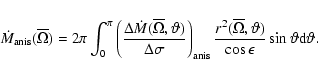 |
(35) |
Indeed, for the anisotropic mass flux we can write
in a compact form
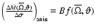 ,
where we put in
the term B all the coefficients which do not depend explicitely
on .
Thus, we have
,
where we put in
the term B all the coefficients which do not depend explicitely
on .
Thus, we have
 |
(36) |
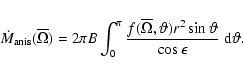
Now, we impose
 |
(37) |
and in this way we can fix the value of B in Eq. (36)
in a manner which is consistent with our definition of
in
Eq. (2). In the numerical calculations we have checked
that with these prescriptions the star is losing exactly the same amount of mass
in the corresponding isotropic and anisotropic cases.
Now, with these various equations,
we can express
in
Eq. (20), which is necessary for
the time dependent outer boundary condition
(Eq. (19)).
Up: Stellar evolution with rotation
Copyright ESO 2002