3 Comparisons with previous theoretical works

 

 

Table 1: Comparisons between modelling parameters for Heasley and co-workers and this work.

	hydrogen		helium
	Heasley et al.	here	Heasley et al.	here
Number of levels	5+1 (HMP, HM2)	20+1	15+4+1	29+4+1
in the model atom	35+1 (HM3)
Frequency redistribution
in resonance lines	complete (CRD)	partial (PRD)	complete (CRD)	partial (PRD)
Detailed balance	Lyman lines	Lyman lines with $n\,>\,5$	resonance lines	no
Detailed incident profile	no	10 lines with upper level $n \le 5$	no	2 lines (584 Å, 304 Å)

It is interesting to compare our results to the pionnering work done by Heasley and his colleagues. We again emphasize that we have removed some restrictive simplifications that were made in their calculations such as the complete redistribution in frequency (CRD). Partial frequency redistribution (PRD) is considered in our calculations for the two first hydrogen Lyman lines and for He I$\lambda$584 Å and He II$\lambda$304 Å. In addition, we use frequency-dependent incident line profiles for the principal transitions (see Table 1). Heinzel et al. (1987) have shown that in the case of hydrogen the combined use of these detailed incident profiles with PRD may change drastically the emitted profiles.

3.1 Heasley, Mihalas, & Poland (1974)

 

 

Table 2: Comparison of physical properties for HMP models. Units: electron temperature T ($^\circ$K); total hydrogen density $n_{\rm H}$(cm^-3). Population ratios are given at the surface and at the center of the slab.

			Optical Depth (total slab)				$n_{He {\sc ii}}/n_{He {\sc i}}$		$n_{He {\sc iii}}/n_{He {\sc ii}}$
Model	T	$n_{\rm H}$	$\tau ^{912}$	$\tau ^{504}$	$\tau_0^{584}$	$\tau ^{227}$	surface	center	surface	center
HMP 1	6000	1010	2.6+0	3.8+0	2.2+4	8.-1	4.-1	3.-1	1.-4	8.-5
here			1.1+1	4.2+0	2.8+4	1.-1	3.-1	7.-2	1.-2	9.-3
HMP 3	6000	1012	3.6+3	1.0+3	3.0+6	1.5+2	1.-2	1.-10	4.-6	1.-16
here			3.9+3	4.8+2	3.1+6	6.-3	2.-2	1.-11	4.-4	3.-6
HMP 7	8000	1010	2.3+0	3.4+0	1.7+4	8.-1	5.3-1	4.6-1	2.-4	1.-4
here			7.8+0	3.8+0	2.2+4	1.-1	4.2-1	1.1-1	1.-2	1.-2
HMP 9	8000	1012	2.2+3	8.8+2	2.4+6	1.3+2	1.-2	3.-7	4.-6	3.-16
here			1.9+3	4.0+2	2.2+6	3.-3	2.-2	5.-8	4.-4	4.-6

 

 

Table 3: Comparison of optical properties (HMP models). Integrated helium line intensities (ergs cm^-2 s^-1 sr^-1).

			$\lambda$ (Å)
Model	T	$n_{\rm H}$	304	537	584	3889	5876	6678	7065	10830
HMP 1	6000	1010	341	8	356	235	1844	61	222	8438
here			906	5	134	170	1300	21	164	6190
HMP 3	6000	1012	132	4	54	73	567	6	69	2625
here			414	5	117	86	661	12	83	3140
HMP 7	8000	1010	424	9	370	259	2032	61	245	9300
here			1100	6	154	197	1500	26	190	7160
HMP 9	8000	1012	150	4	65	102	784	9	95	3615
here			431	6	134	60	449	20	56	2110

The first paper of the series (HMP) considers hydrogen and helium (neutral and ionized) spectra emitted by the same geometrical prominence model as described above. The dilution factor for all lines and continua is taken to be $\frac{1}{2}$, corresponding to a zero altitude. They use a 15+4+1 helium atom. Levels for He I with quantum number n=4 and n=5 are included as grouped L states, keeping the distinction between singlet and triplet states. Collisional rates are given by Mihalas & Stone (1968), and Auer & Mihalas (1973) give collisional rates not included in Mihalas & Stone (1968) as well as photoionization rates. Oscillator strengths are obtained from Wiese et al. (1966). No turbulent broadening is considered, and CRD is assumed. HMP have adopted a relation which defines the radiation temperature as a function of wavelength for the incident radiation for continuum points (see their Fig. 1). But their relation was inaccurate for the continuum incident radiation shortward of 304 Å. They indeed extrapolated EUV fluxes for the He II resonance continuum from OSO-4 and OSO-6 spectrometers which had a wavelength cutoff at about 300 Å. In all our calculations we therefore use EUV fluxes given by Heroux et al. (1974) that give more ionizing radiation in the He II resonance continuum. No emergent profile is shown in their paper. Table 1 lists the main differences between their computations and our code.

We indicate in Tables 2 and 3 some comparisons for four computed models, which all have a slab thickness of 6000 km at height H=0 km, temperatures of 6000 (models HMP 1 and 3) and 8000 K (models HMP 7 and 9), and mean hydrogen densities of 10¹⁰ (models HMP 1 and 7) and 10¹² cm^-3 (models HMP 3 and 9). Table 2 presents the comparisons for the optical depths at the head of the Lyman continuum ( $\tau ^{912}$), of the He I continuum ( $\tau ^{504}$), of the He II continuum ( $\tau ^{227}$), and at the 584 line center ( $\tau_0^{584}$), as well as the population ratios $n_{He {\sc ii}}/n_{He {\sc i}}$ and $n_{He {\sc iii}}/n_{He {\sc ii}}$. Table 3 shows the results for the integrated intensities of the He II $\lambda$304 Å line and several neutral helium lines.

One can note a rather good agreement between the two computations, except for the population ratios $n_{He {\sc iii}}/n_{He {\sc ii}}$ and $\tau ^{227}$. At high densities a large disagreement occurs for those quantities. This discrepancy is mainly due to the different incident continuum radiation in the He II resonance continuum. We have an ionization continuum which is much more efficient to populate He III. Examination of $\tau ^{504}$ and $\tau_0^{584}$ indicates that the neutral helium populations are of the same order in both works. At low densities we have less He II and more He III than HMP. The increase of pressure leads to lower $\tau ^{227}$ in our computations but has the opposite effect in HMP calculations. This implies that the penetration of the EUV ionizing radiation is much more effective for our models. The result is that we get a much larger He III population in the slab. The integrated intensities in Table 3 reflect this situation. The neutral helium line intensities are roughly of the same order in HMP calculations and ours, but the He II $\lambda$304 Å line intensity is systematically higher in our computations. At those high pressures fast recombinations from the He III ionization level follow the photoionization of the He II ground state. Radiative cascades towards the ground level of He II then occur, thus producing a strong emission in the 304 resonance line. Nevertheless the high densities of HMP models imply high pressures of about 1 dyn/cm² and more which should not be regarded as very representative of the actual pressures in quiescent prominences.

   
3.2 Heasley & Milkey (1978)

Figure 3: $E({\rm D}3)$ (top) and $E(6678)/E({\rm D}3)$ (bottom) versus $E({\rm H}\beta )$ for 3 models of HM3. Dashed lines are calculations by HM3, and solid lines represent our results. The three kinds of models are: 7500, 0.01 (+); 9000, 0.015 ($\ast$); 7500, 0.02 ($\Diamond$). Integrated intensities are in cgs units.

HM3 presented new computations of hydrogen and helium emerging spectra for more realistic models with more realistic temperature and pressure values as compared to HMP, new continuum incident intensities of Heroux et al. (1974), and lower dilution factors for the incident radiation. This was necessary for the authors in order to match the prominence observations made available by Landman & Illing (1977). Unfortunately they do not give the new dilution factors that they adopted. We therefore use a dilution factor corresponding to an altitude of 10000 km, viz. 0.416 (if there is no center-to-limb effect). CRD is still assumed for all lines and continua. Moreover they have solved the statistical equilibrium equations with the assumption that all Lyman lines are in detailed radiative balance. No emergent profiles and no quantities related to He II are given. 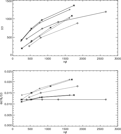HM3 studied the triplet line D3 and the 6678/D3 singlet-triplet line ratio. Figure 3 presents comparisons between HM3 results and our computations for $E({\rm D}3)$ and $E(6\,678)/E({\rm D}3)$ versus $E({\rm H}\beta )$ for three classes of models without microturbulent velocity and defined by the temperature and the pressure: (7500, 0.01); (9000, 0.015); (7500, 0.02) - see their Figs. 4 to 6. In each model different calculations were made for column masses of $2\times 10^{-6}, 4 \times 10^{-6}, 6 \times 10^{-6}$, and $1.2 \times 10^{-5}$ g/cm². We can notice that our $E({\rm D}3)$ are larger in every case than those of HM3. This seems to be due to a better penetration of the ionizing incident radiation in our models since helium recombination tends to populate the triplet levels. We also recall the uncertainty in the dilution factors that they used for the incident radiation. The relation between $E({\rm D}3)$ and $E({\rm H}\beta )$ is studied in Sect. 5.5 for a larger number of models. On the other hand the ratio $E(6\,678)/E({\rm D}3)$ is lower in our computations than in HM3. Again the better penetration of the incident continuum explains this situation since ionization of helium hardly affects the singlet states populations but populates the triplet states through recombination. Moreover, the ratio $E(6678)/E({\rm D}3)$ varies much less in our computations, especially for the (7500, 0.02) models. It indicates that the line formation processes for both the D3 and the 6678 lines are not altered with the increase of the H$\beta$ intensity, or in other words they do not change much with the increase of hydrogen column mass in this domain of temperatures and pressures. The main contribution in the line formation comes from the scattering of the incident radiation. Of course, absolute intensities increase with the hydrogen column mass. We will see in Sect. 5.3 (Fig. 18) that the relation between E(6678) and $E({\rm D}3)$ strongly depends on the temperature and the pressure.