5 Classification of stellar oscillations

To discuss the differences between the new classification scheme proposed in this work relatively to the classification schemes normally used, we present in the following the original classification proposed by Cowling (1941) and the generalization of that one made by Eckart (1960), Scuflaire (1974) and Osaki (1975).

5.1 Classical classification schemes

The first classification scheme to label the eigenmodes of oscillations was introduced by T. Cowling (1941). This is valid provided that the reduction of the fourth-order system of nonradial adiabatic stellar oscillations to a second-order system is obtained under the hypothesis that the Eulerian perturbation of the gravitational field can be ignored. This scheme provides a good qualitative description of higher-order modes for l=0 and l=1 and for all the modes with $l \ge 2$.

Formally, the frequency is unbounded below (except when l=0), and also unbounded above. Therefore, it is not immediately obvious where to choose the origin of n. It is possible to choose n such that as $n\rightarrow \pm \infty$for a fixed l, |n|-1 is the number of zeros in the eigenfunction, when $l \ge 2$ and |n| is the number of zeros in the eigenfunction, when l = 0. For spherically symmetrical modes (l=0), the lowest-frequency mode (fundamental mode) is labeled n=1. In simple stellar models, modes with n >0 and n <0 have the characteristics of acoustic and internal gravity waves; they were designated p-modes and g-modes by Cowling (1940). Modes with n=0, are fundamental g-modes or f-mode, and have the property that when $l \gg 1$, they have no zeros in the eigenfunction. Under these considerations, the modes of a star can be classified as p-modes for n>0 and g-modes for n<0, and a (unique) f-mode for n=0. Then both g and p sequences start from n=1. The fundamental l=0 mode, was labeled with n=1.

The Cowling classification scheme has been generalized by Eckart (1960), by taking into account the tunnel effect that can take place when the competition between the two restoring forces pressure and gravity is of the same order. Eckart (1960) discusses how the phase differences between vertical displacement and pressure fluctuation decreases with height for acoustic modes and increase for g-modes, so that order n can be computed by first assigning a signal to each zero in the eigenfunction according to the direction of variation of the phase difference, and then counting the zeros algebraically. Scuflaire (1974) and Osaki (1975) presented the same criterion to classify stellar oscillations. Scuflaire (1974) has demonstrated that, for relatively condensed polytropic modes $n_{\rm e}\ge 3.4213$ (in case of modes of degree l=2) and $\gamma =5/3$, the mixing of modes (in the Cowling approximation) occurs. This classification scheme, has been found to work well in most stars for oscillations with $l \ge 2$, when the Cowling approximation is not considered. The problem remains for l=1. Another classification scheme was proposed by Shibahashi & Osaki (1976), based on the properties of the wave on the main trapping region.

However, none of these classification schemes is sufficiently general. This is due to two main reasons. One, is the fact that the classification scheme is dependent on the eigenfunction used to determine the order n of the mode, which in the most general case does not necessarily have the same number of zeros of other eigenfunctions choosen also to classify the modes of some physical system (Cox 1980). This means that the classification scheme depends on the properties of the wave function choosen to define the system, as it has been illustrated by different authors (Cox 1980 and references there). The classification scheme does not work for modes with $l \le 1$. Even if we consider that this hypothesis is acceptable, there is a second problem which remains. It is the fact that all the classification scheme has been done under the Cowling approximation, and the full problem is just an extension of this case.

5.2 New classification scheme

The resonant cavities are clearly defined for all modes of any order, and not only for modes of high-order and very high degree, as is normally done in the most classical scheme classifications. We start by pointing out, that the phase functions $\theta_i(l,\omega;r)$, only depend on the structure of the equation of motion, i.e. on the topology of the propagation diagram.

The oscillation corresponding to an eigenstate, can be defined in terms of the boundary conditions, where $\omega ^2$ is a parameter. In this sense, an eigenstate occurs when the difference of phase between the initial phase at r=0and the final phase at r=R, are a multiple of $\pi$. This introduces a natural scheme classification for the eigenmodes, which determines the order number of the mode, n, as the integer associated to the total number of $\pi$-cycles that the phase function has developed from the inner endpoint where the inner boundary condition is fixed until the outer endpoint where the outer boundary condition is fixed (see Sect. 4). The determination of the eigenvalue equation, similar to the Bohr-Sommerfeld quantization rule, is done in one particular description given that, as we mentioned previously, both descriptions are equivalent. An eigenstate corresponds to the following condition for each of the wave types:

$$\phi (\omega,l,R)=\theta_i(\omega,l;R)-\theta_i(\omega,l;0)=n\pi$$ (56)

where $\phi(\omega;R)$ is the difference between the outer boundary condition fixed for r=R, given by $\theta_i(\omega,l;R)$and the inner boundary condition given by $\theta_i(\omega,l;0)$. In our case it is given by the expression 47 (or 48). n, is a negative or positive integer, starting from 0. The well-ordered sequence of eigenfrequencies, corresponding to the ordering of the integer n, from $-\infty$ to $+\infty$, is guaranteed by the properties of the phase function discussed in the last section. The only exception is the unique f-mode. It will be positive, if $\theta_i (R,\omega)> \theta_i(0,\omega)$ and it will be negative in the opposite case. The negative integer is reserved for the gravity modes, and the positive integer for the acoustic modes. However in the case of mixed modes the sign of n, determines the dominant character of the propagation mode. This classification scheme is general and is fixed by the boundary conditions, and does not depend on the turning points of the modes, or even on the algebraic counting of the number of nodes of the eigenfunction (i.e. the number of $\pi$ cycles, that the phase function has developed from the internal endpoint, until the external endpoint).

The more condensed polytropes (see Fig. 2b) cannot have the f-mode. However, the degeneracy of the eigenstates of low order modes can occur more frequently due to the overlap of the two propagative regions. In Figs. 3 and 4 we present the propagation diagram and the linear phase diagram of a polytope of index $n_{\rm e}=3$. The high values of |n| correspond to pure acoustic waves for positive values of n and pure gravity waves for negative values of n. This occurs because these waves present only one propagative region and a well behaved phase function in each case. In that case, the main properties are conserved for modes of low radial order. However, in the case of condensed polytropes such as polytropes of index $n_{\rm e}=4.5$, for the lower radial order modes, the wave function presents a mixed character which is determined by each of the two propagative regions. In this case the eigenstate can occur by two possible ways: or the eigenstate is mainly determined in only one of the propagative regions, or is fixed by both propagative regions when the evanescent region between them is small compared with the wavelength of the wave, i.e., tunnel effect. It will be the particular topological nature of the propagation diagram that will determine the different eigenstates. In such cases the previous classification fails for modes of low degree, particularly those with l=1, in highly condensed stellar models. In the scheme presented, the dipole modes have a perfect ordering, even for the lowest orders, such as $n \le 2$. This is evident for modes of a polytrope of index $n_{\rm e}=4$ with $n \le 3$, l=1 (see Fig. 5). The lower-order modes have phase paths quite different from those of the higher-order modes, because the perturbation to the gravitational potential in the central region can change the character, in regions where the mode behaves like a gravity wave. We believe that this is the reason why previous classification schemes do not work. This behaviour is likely to occur in real stars (Lopes 2000).

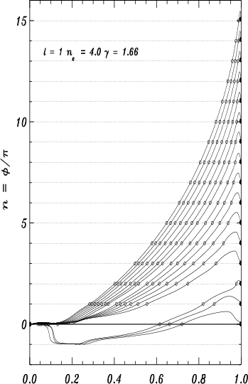Figure 5: Linear phase diagram of modes of degree l=1, for a polytropic model of index, $n_{\rm e}=4$ and adiabatic index $\gamma =5/3$. The representation adopted is the same of the previous figure.

It is convenient, also to point out the agreement between this method and the classical method proposed by Cowling (1941) and others, for the higher order modes of simple stars (see Fig. 4). For example, for a polytrope of $n_{\rm e}=3$the eigenstate of order n=10, corresponds to an acoustic mode, for which the phase function, presents 11 nodes (i.e. $\pi$-cycles of the phase function) and is classified with n=10 in the classical scheme. A gravity wave, of order n=6presents 7 nodes and is classified with n=6 in the classical scheme.

Finally, we observe that only in the case of a Sturm-Liouville eigenvalue type problem, it is guaranteed that the eigenfunction associated to some eigenvalues, has exactly n zeros (Cowling 1941). It is just in eigenvalue problems similar to that one that it is possible to use the counting of the zeros of the eigenfunction to label the order of the eigenstate. Moreover, the algebraic counting of zeros of the eigenfunction on the gravity region or the acoustic region can also be used to label the states of the system (Scuflaire 1974). This is on the basis of the usual classification schemes, and it is one of the reasons why they do not work.