Initially, it should be natural to assume that surveys with different filter sets show quite a different performance in terms of classification and redshift estimation. If a survey aims for objects with very particular spectra, the filter set can certainly be tailored to this purpose. If the objects of interest span a whole range of spectral characteristics, it is not trivial to guess via analytic thinking which filter set performs best.
Originally, this method was developed for CADIS using real CADIS data to test it. Then, we intended to optimize it and try to draw conclusions about survey strategies. Aiming for more insight into the question of filter choice, we performed Monte-Carlo simulations on different model surveys by feeding simulated multi-color observations of stars, galaxies and quasars into our algorithm. Here, we present a comparison of three fundamentally different filter sets and show their resulting performance for classification and redshift estimation.
The three model surveys spend the same total amount of exposure time on different filter sets, but use the same instrument, telescope and observing site. We chose the Wide Field Imager (WFI) at the 2.2-m-MPG/ESO-telescope on La Silla as a testing ground, because it provides a unique, extensive set of filters ranging from several broad bands to a few dozen medium bands to choose from. Furthermore, the WFI is a designated survey instrument which is extensively used by the astronomical community.
 /fwhm (nm) /fwhm (nm) |
name |
 |
 |
 |
| 364/38 | U | 23.5 | 23.5 | 24.1 |
| 456/99 | B | 25.0 | 25.0 | 25.6 |
| 540/89 | V | 24.5 | 24.5 | 25.1 |
| 652/162 | R | 24.5 | 24.5 | 25.1 |
| 850/150* | I | 23.0 | 23.0 | 23.6 |
| 420/30 | 23.6 | 23.98 | ||
| 462/14 | 23.5 | |||
| 485/31 | 23.4 | 23.78 | ||
| 518/16 | 23.3 | |||
| 571/25 | 23.2 | 23.58 | ||
| 604/21 | 23.1 | |||
| 646/27 | 23.0 | |||
| 696/20 | 22.8 | 23.18 | ||
| 753/18 | 22.7 | |||
| 815/20 | 22.6 | 22.98 | ||
| 856/14 | 22.5 | |||
| 914/27 | 22.4 | 22.78 |
The three modelled surveys, here called setup "A'', "B'' and "C'', each spend 150ksec of exposure time distributed on the following filters (see also Table 1):
Setup A spends 50ksec on the five broad-band filters of the WFI (UBVRI) and
100ksec on twelve medium-band filters. Using ESO's exposure time calculator V2.3.1
for the WFI, we related exposure times to limiting magnitudes assuming a seeing of
 ,
an airmass of 1.2, point source photometry and a night sky illuminated by
a moon three days old. The exposure times are distributed such, that a quasar with a
power-law continuum
,
an airmass of 1.2, point source photometry and a night sky illuminated by
a moon three days old. The exposure times are distributed such, that a quasar with a
power-law continuum
 and a spectral index of
 is
observed with a uniform signal-to-noise ratio in all medium bands. As a result, the
twelve medium bands each deliver a 10-
is
observed with a uniform signal-to-noise ratio in all medium bands. As a result, the
twelve medium bands each deliver a 10- detection of an R=23.0-quasar.
Setup B spends 50ksec on the same broad bands but concentrates the 100ksec for
medium-band work on only six filters reaching a uniform 10-
detection of a
R=23.38-quasar then.
Setup C finally spends all 150ksec on the broad-band filters and omits the medium bands entirely.
In Sects. 4.2 and 4.3 we present the performance results for setup A, which has actually been used for a recent multi-color survey (Wolf et al. 2000). The relative performance of the three setups is compared in Sect.4.5. In Sect.4.6 we attempt to derive some basic analytic conclusions.
The simulations are carried out by creating a list of test objects from the color libraries presented in Sect.3. We assume a certain R-band magnitude and calculate the individual filter fluxes and corresponding errors for each object. Then we scatter the flux values of the objects according to a normal distribution of the flux errors. Finally, we recalculate the resulting color indices and index errors and use this object list as an input to the classification.
For the stars we use just 131 test objects as there are members in the library. For the test galaxies we take only every third member of the present library giving us 6700 objects. From the quasar library we use every seventh object resulting in 6450 quasars per test run.
These simulations show us how well the classification can possibly work, assuming that real objects will precisely mimic the library objects. Every real situation will contain differences between SED models and SED reality, sometimes called "cosmic variance'', which will worsen the performance of every real application. Nevertheless, the simulation highlights the principal shortcomings of the method itself and the chosen filter set in particular. Therefore, it can be used to judge the relative performance of different filter sets.
We run these tests for stars, galaxies and quasars with magnitudes of R= 22, 23, 24
and 25, respectively, in order to see how the classification performance degrades
from optimum to useless with decreasing object flux. Given that R=23 corresponds
roughly to the 10-
limit of setup A, the most shallow survey, we expect that
the classification has almost reached its best performance at R=22. This is due to
our assumption of a 3% uncertainty in the calibration, which causes even the
brightest objects with the best photon statistics to perform not much better than an
object detected only at a 30-
level. Finally, at R=25 objects are well
detected only in the broad-band filters, while the medium bands yield only fluxes
with errors higher than 40%. We expect the surveys to be almost useless at this
level.
| R=23 | true class, setup A | true class, setup C | ||||
| classified as | star | galaxy | quasar | star | galaxy | quasar |
| star | 0.98 | 0.96 | 0.03 | |||
| galaxy | 0.01 | 0.95 | 0.01 | 0.01 | 0.92 | 0.01 |
| quasar | 0.01 | 0.94 | 0.84 | |||
| unclassified | 0.01 | 0.04 | 0.05 | 0.03 | 0.08 | 0.12 |
We now look at the classification performance as achieved in setup A, the model survey with the highest number of filters, but the shallowest exposures in terms of photon flux detection:
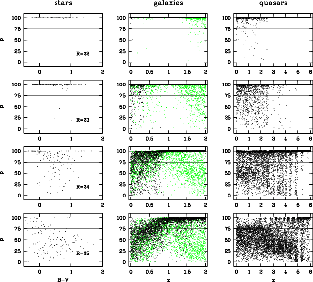
For R=22 it turned out, that the classification works almost perfect (see uppermost row of diagrams in Fig.5). Generally, more than 99% of all test objects in any class are correctly classified.
At R=23, usually less than 5% of all objects in any class get lost to
unclassifiability. Most affected with 10% incompleteness are quasars at z<2.5 with
red spectra and weak emission lines. In this simulation, their location in color
space overlaps with starburst galaxies at redshift 1.6<z<2.0. So far, our galaxy
templates contain no information in the spectral range bluewards of the
Lyman- line leaving their U-band flux blank in this redshift range. As a
result, the classification omits this band for the comparison with the library
galaxies.
line leaving their U-band flux blank in this redshift range. As a
result, the classification omits this band for the comparison with the library
galaxies.
At R=24, about one third of the stars get lost. These are mostly yellow stars which are too faint in every filter to be classified unambiguously. Rather blue and rather red stars are still successfully classified, because either on the blue or on the far-red side of the filter set they still show significant fluxes and sufficiently accurate color indices. About a quarter of the galaxies would be missed, which are either blue galaxies not showing strong continuum features or red galaxies at redshifts low enough to render them faint in the far-red filters, too. Also, a quarter of the quasars is lost, either red z<2.5-quasars overlapping again with starburst galaxies at 1.6<z<2.0, or z>2.5-quasars with weak emission lines overlapping with early-type galaxies at z<0.4.
At R=25, the classification has finally become highly incomplete, but can still find very blue stars and very red extragalactic objects like quiescent galaxies and quasars at higher redshift (see bottom row in Fig.5, see also Fig.9 for precise numbers).
In all simulations, most incorrectly classified objects are unclassifiable and a minority of them are scattered into another class (see also classification matrix, Table 2). Especially, quasars seem to be not strongly contaminated by false candidates. At any magnitude in any setup, less than 1% of the galaxies are scattered into the quasar candidates except for setup C at R=25. Still, this contamination in the quasar class is not negligible, since a minor fraction of a rich class can be a large number in comparison with a poor class. In CADIS we found about 3% of the extragalactic objects at R<23 to be quasars. A contamination of less than 1% means that less than a quarter of the quasar candidates should be galaxies.
Figure 6 displays the comparison of the photometric MEV+ redshift estimates in setup A with the original true redshifts of the simulated objects. At R=22 (see uppermost row of Fig.6) the redshifts work quite satisfactorily for galaxies and quasars, which is demonstrated by nearly all objects residing on the diagonal of identity.
Towards fainter magnitudes, the galaxy redshifts degrade first at both the lower and
the higher redshift ends. The deepest working magnitudes are reached in the redshift
range of 0.5<z<1. This feature is due to the location of the 4000Å-break: When
the break is located in the central wavelength region of the filter set, many filters
are available on either side of the break to constrain its location rather well even
for noisy data. For
 ,
the 4000Å-break is at least enclosed by
mediumband filters. But if the break is located close to the edge of the filter set
and, e.g., detected only by a noisy signal from a single filter, the true redshift
interpretation can not be distinguished well from other options.
,
the 4000Å-break is at least enclosed by
mediumband filters. But if the break is located close to the edge of the filter set
and, e.g., detected only by a noisy signal from a single filter, the true redshift
interpretation can not be distinguished well from other options.
Quiescent galaxies still work reasonably fine at the higher redshift end, because they are brighter in the far-red filters. Starburst galaxies mostly degrade at higher redshift, because they have less discriminating (and trustworthily known) features in the UV than in the visual wavelength range.
The quasar redshifts remain rather precise at
 ,
all the way down to
R=25. This is the redshift range, where the continuum step over the Lyman-line can be seen by the filter set and redshift estimates are expected to reach deep.
Of course, at
,
all the way down to
R=25. This is the redshift range, where the continuum step over the Lyman-line can be seen by the filter set and redshift estimates are expected to reach deep.
Of course, at
 the R-band magnitude of quasars appears artificially faint,
since it is strongly attenuated by the Lyman-
forest, but the redder filters
contain higher flux levels sufficient to constrain the location of the continuum
step. Redshift confusion arises first in the low-redshift region working its way up
to higher redshifts with decreasing brightness. At z<2.2 the continuum shows no
Lyman-
forest in our filter sets, but only a redshift invariant power-law
shape. In this case, the multi-color redshifts rely solely on some emission-lines
showing up in the medium bands.
the R-band magnitude of quasars appears artificially faint,
since it is strongly attenuated by the Lyman-
forest, but the redder filters
contain higher flux levels sufficient to constrain the location of the continuum
step. Redshift confusion arises first in the low-redshift region working its way up
to higher redshifts with decreasing brightness. At z<2.2 the continuum shows no
Lyman-
forest in our filter sets, but only a redshift invariant power-law
shape. In this case, the multi-color redshifts rely solely on some emission-lines
showing up in the medium bands.
Some concentrated linear structures are visible off the diagonal at lower redshift
with the best contrast at R=24. Their origin is a misidentification of weak
emission lines: There are two structures mirrored at the diagonal following the
linear relations
 and
and
 .
They are caused by a confusion of the MgII line with the H
.
They are caused by a confusion of the MgII line with the H line.
Another structure at
line.
Another structure at
 arises from weak
Lyman-
lines of very blue quasars which are interpreted as CIV lines, or
weak CIV lines which are taken to be CIII lines. The extent of these structures
across the diagram obviously depends on the visibility of the involved lines within
the medium-band filter set. Finally, there is a large group of quasars estimated to
be at nearly zero redshift, but truely strechting even beyond z=3. These are among
the quasars with the lowest emission line intensities in the library, which basically
display only their redshift-invariant power-law continuum in the filters.
arises from weak
Lyman-
lines of very blue quasars which are interpreted as CIV lines, or
weak CIV lines which are taken to be CIII lines. The extent of these structures
across the diagram obviously depends on the visibility of the involved lines within
the medium-band filter set. Finally, there is a large group of quasars estimated to
be at nearly zero redshift, but truely strechting even beyond z=3. These are among
the quasars with the lowest emission line intensities in the library, which basically
display only their redshift-invariant power-law continuum in the filters.
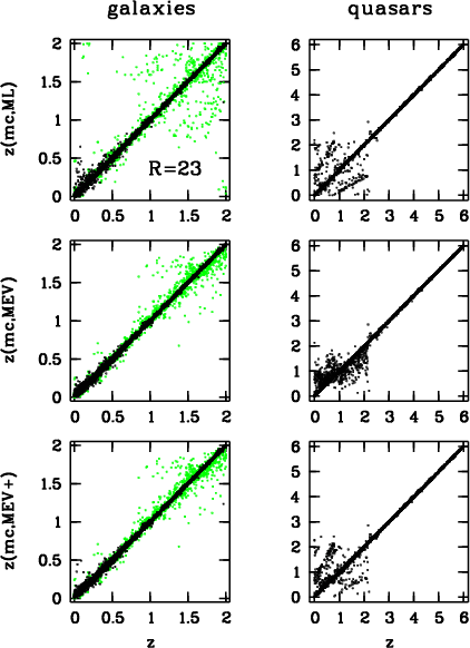
We now compare the relative performance of three different redshift estimators using the example of galaxies and quasars at a fixed magnitude of R=23. We have used the Maximum Likelihood (ML) method, the Minimum Error Variance (MEV) method and an advanced MEV method (MEV+) as we defined it in Sect.2.4.
While the Maximum Likelihood (ML) method always gives a redshift estimate, the Minimum Error Variance (MEV) method does not in the way we use it. Some objects have probability distributions which are close to flat yielding a redshift estimate that reflects primarily the redshift interval chosen for the template library rather than giving a reliable physical interpretation of the object. We do not assign any estimate to these uncertain objects (as we defined them in Sect.2.4), which is justified with their estimates being senseless anyway. A caveat for a direct performance comparison is the fact, that the MEV/MEV+ methods ignore the uncertain objects, whose selection function is redshift-dependent at the faint end and could furthermore be different in a real dataset due to cosmic variance.
As shown in Fig.7, the different estimators deliver rather comparable results with quite similar redshift accuracy. In case of the quasars the improved MEV+ method (which can detect bimodal probability distributions) performs different from the standard MEV method but rather similar to the ML method. This is due to bimodalities where the MEV estimate is a weighted average of the two present probability peaks, while the MEV+ estimate decides for the single peak containing the higher probability integral, which is likely to be roughly coincident with the ML estimate pointing at the redshift with the highest individual probability. Bimodalities can again be seen as linear structures off the main diagonal and arise from confusion among emission lines. In case of the pure MEV method the peak associated with the wrong solution is averaged with the correct solution residing on the diagonal, and the MEV plot shows smeared out structures around the diagonal rather than the linear ones like the ML or MEV+ plots.
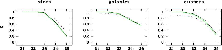
All setups are designed to spend the same amount of exposure time on a survey field, but distribute it on different filter sets. The pure broad-band survey, setup C, collects far more photons than the setups A and B, which are mainly exposing medium-band filters. But due to their higher spectral resolution, we expect setups A and B to contain more information per photon.
In fact, it turns out, that the classification performance of all three setups is quite similar, which implies that the lack of photons in the medium bands is pretty much compensated by their higher information content (see Fig.9). Among the small remaining differences, there is a tendency for the medium-band setups to be more efficient in finding quasars, supposedly because their spectra contain emission lines which are more prominent in narrow filters.
Also, there is a slight trend indicating that the medium-band surveys sustain a high level of completeness to somewhat fainter magnitudes and then drop more sharply than setup C. In the incompleteness range of very faint magnitudes, all setups perform rather equally meager.
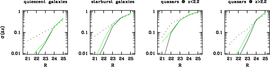
The same trends are more clearly present among the multi-color redshifts, where we
compare the statistics for the ML estimator (see Fig.10): Setups A and B
provide a much better redshift resolution at the usual working magnitudes. They only
fall behind the performance of setup C by a rather insignificant degree in the
faintest regime, where the redshift estimates are close to unusable to start out
with. This advantage of setup C results just from the broad bands being deeper by
 ,
where the medium-band filters do not contribute to the result anymore.
,
where the medium-band filters do not contribute to the result anymore.
For brighter objects, estimates in setup A are better than in setup B by an average
factor of two, just reflecting the difference in spectral resolution. After all, the
convolution of any measurement with a 0
 03-Gaussian (to account for the calibration
errors) makes better photon statistics useless among objects, which are detected at
more than a
03-Gaussian (to account for the calibration
errors) makes better photon statistics useless among objects, which are detected at
more than a 
 -level. Thus, only increasing the number of filters
improves the result for these objects while increasing the depth of any filter has no
effect.
-level. Thus, only increasing the number of filters
improves the result for these objects while increasing the depth of any filter has no
effect.
At this point we like to emphasize, that the calibration uncertainty limits the best
achievable performance. We stress, that a large calibration error of e.g. 10% would
turn an entire survey catalog into a collection of "less-than-10--objects'',
at least within our method. If calibration is expected to be a problem due to
instrumentation or observing strategy, this conclusion strongly suggests that a large
number of filters giving many noisy datapoints deliver more information than a few
long exposed and formally deep filters that can not exactly be matched together.
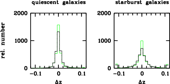
Once more we look into the details within classes: it is no surprise that quiescent
galaxies with rather prominent 4000Å-breaks receive more accurate redshift
estimates than starburst galaxies with less contrasty continuum features. When
comparing equal accuracies, we find that estimates for quiescent galaxies reach
typically one magnitude deeper than for starburst objects. When aiming for a redshift
resolution of
 among quiescent galaxies, it is interesting to
see, that any of the medium-band surveys reaches two magnitudes deeper than the
broad-band survey (setup C).
among quiescent galaxies, it is interesting to
see, that any of the medium-band surveys reaches two magnitudes deeper than the
broad-band survey (setup C).
The quasar redshifts work best at z>2.2, when the estimation depends not only on
emission lines but can take advantage of a strong continuum feature being present
within the range of the filter set, i.e. the continuum suppression bluewards of the
Lyman-
line. As in the case of galaxies, setups A and B have significantly
stronger resolving power in terms of redshift than setup C, with setup A again being
the best choice.
It is inspiring to conclude from these simulations, that photometric redshifts for
quasars are feasible and are supposed to reach accuracies of
 in
surveys with medium-band filters. Furthermore, observations from the CADIS survey
find a surprising number of faint quasars, whose multi-color redshifts were indeed
proven by spectroscopy to be as accurate as expected from the simulations (see Wolf
et al. 1999 and Paper II).
in
surveys with medium-band filters. Furthermore, observations from the CADIS survey
find a surprising number of faint quasars, whose multi-color redshifts were indeed
proven by spectroscopy to be as accurate as expected from the simulations (see Wolf
et al. 1999 and Paper II).
Altogether, setup A seems to be the most successful among the ones discussed for photometric classification and redshift estimation. It has no disadvantages compared to the other setups, especially it does not lack working depth compared to the pure broad-band survey. Viewing the almost vanishing differences between setup A and B, there might be no incentive to increase the number of filters even higher.
Still, setup A shows a selection function for a successful classification with some redshift dependence. Among the quasars shown in Fig.5, we can see some vertical stripes containing objects at selected redshifts, which are not successfully classified anymore, while the neighboring redshifts still work well. In principal, a set of neighboring medium-band filters touching in wavelength and covering the important spectral range completely would most likely result in a selection function with the smoothest shape and smallest redshift dependence.
In this section, we would like to address the issue of choosing an optimal filter set by analytic thoughts based on a simplified picture of the classification problem. We assume, that we are still limited by a fixed amount of telescope time, which we can distribute over some filters. If different wavebands could be imaged simultaneously, it would be obvious that even a faintly exposed full-resolution spectrum would be better than an unfiltered white light exposure, as long as read-out noise of the recording detector is not an important constraint. Here, we want to discuss the less obvious scenario of consecutive exposures in different wavebands.
As mentioned in the introduction, the choice of the optimum filter set depends entirely on the goal of the survey. For surveys aiming at a particular type of objects with characteristic colors, tailored filter sets can be designed. But if we intend to integrate different survey applications into one observational program on a common patch of sky, then we need a single survey to identify virtually every object unambigously. In this scenario two choices have to be made:
We first note, that if all colors were equally discriminating for each object, the choice would be arbitrary. Any distribution on any number of equally wide filters would provide the same total discriminative power and classification performance. In practice, objects can reside at many different redshifts and usually only part of their spectra have discriminating features.
We now try to obtain some insight into this question based on very basic template assumptions. For simplicity, we now just assume two different possible objects posed to the classification algorithm, with one of them being a quasar only distinguished by an emission line from another object with an otherwise identical spectrum.
Addressing choice (1), we find, that concentrating on few filters would mean that only few quasars display their emission line in a filter and can be classified correctly down to some limit, while many objects would be unclassifiable. The classification would lack completeness, but reach deep for a few objects. Distributing exposure time among many filters covering the entire spectrum would give every quasar a chance to show its emission line, which implies that every object is well classifiable but not to the same depth. The classification would remain rather complete and degenerate more sharply than in the case of few filters when reaching its limiting magnitude.
Addressing question (2), we assume one of the filters to observe the emission line and evaluate the line contrast obtained. As long as the line is completely contained in the filter bandpass, our signal, i.e. the absolute flux difference to the continuum induced by the line, is a constant value irrespective of the filter width. The noise is given by the square-root of the total flux from the object which increases along with the width of the bandpass. The optimum signal-to-noise ratio is obtained with a filter matching just the width of the emission line. Any narrower filter would cut off line flux, thus shrinking the signal more than the noise.
Using both conclusions we can ask for the optimum strategy when aiming for high
sensitivity and completeness across some redshift range. This goal requires that we
observe the emission line in any case regardless of the redshift. Therefore, we need
n filters to cover the entire spectrum in question, depending on the filter width
 .
Given a fixed total amount of exposure time, the
exposure time per filter and thereby the counts measured from the line are
.
Given a fixed total amount of exposure time, the
exposure time per filter and thereby the counts measured from the line are
 .
The total flux
.
The total flux
 in this filter depends on the same exposure
factor and on
in this filter depends on the same exposure
factor and on
 ,
so that the
,
so that the
 and
and
 .
Therefore, the signal-to-noise ratio
.
Therefore, the signal-to-noise ratio
 const,
independent of the number of filters in any set providing complete coverage.
const,
independent of the number of filters in any set providing complete coverage.
In summary for the simple quasar example, we have a free choice on the filter set, as long as we cover the spectrum. It seems, that the width of the filters does not affect the magnitude limit for a successful classification, but it determines directly the redshift resolution. Having the free choice, many filters tailored to the typical width of quasar emission lines would be the best solution.
Another example is photometric star-galaxy separation. Some red stars display broad-band colors similar to some redshifted early-type galaxies. Good photometric accuracy is required to tell them apart, especially if only few filters are available. With medium-band filters enclosing the redshifted 4000-Å-break of the galaxies and probing the absorption bands of stars, the two classes can easily be discriminated even at rather noisy flux levels.
Let us assume the most general imaginable case for the classification problem, where the object spectra can have features with potentially any location and any width (due to redshift as well as class). The arbitrary location calls for a filter set covering the entire spectrum. Again, we are left with the choice of many narrow versus few broad filters mentioned in the simple quasar example just above. And again, as long as the features are smaller than the filter width, the choice of filters makes no difference to the classification, if the same total amount of telescope time is used.
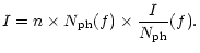
We now consider an abstract information value I obtained by a survey. It depends on
the number of filters n, on the photons collected in each of them
 and
on the information
and
on the information
 that a single photon carries after passing through
a given filter. If on average the same amount of information is obtained in every
filter, we get:
that a single photon carries after passing through
a given filter. If on average the same amount of information is obtained in every
filter, we get:
 |
(29) |
For complete coverage the number n of filters again depends on the filter width
.
Given a fixed total amount of telescope time, the
exposure time per filter is
 and thus the number of photons
collected is
and thus the number of photons
collected is
 .
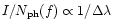
Since narrow filters show features with more
contrast than broad filters, we can assume that the information per photon is
inversely proportional to the filter width:
.
Since narrow filters show features with more
contrast than broad filters, we can assume that the information per photon is
inversely proportional to the filter width:
 ,
and thus
,
and thus
 .
Altogether, the information content of the survey
results to:
.
Altogether, the information content of the survey
results to:
 |
(30) |
In theory, the amount of information in terms of classifiability of objects depends only on the total telescope time and not on the characteristic width of the filters, as long as they cover the entire spectral range in question. The smaller number of photons in the medium-band survey is compensated by the larger number of filters and the higher information content per photon. But this conclusion is based on three simplified assumptions:
In practice, there are several advantages for medium-band and mixed surveys compared to broad-band surveys, especially when combined with our classification scheme:
Especially the last three advantages can cause a medium-band survey to reach even deeper than a broad-band survey in terms of classification and redshift estimation, although its nominal flux detection limits might have suggested inferior performance to the intuitive judgement.
The disadvantage of a survey project involving many medium-band filters is, that it needs a larger minimum amount of telescope time, since a few constraints in observational strategy have to be met. An optimal survey has requirements for:
Copyright ESO 2001
 .
The probability for a simulated object to be
assigned to its original class is plotted over the color B-V for stars and over the
redshift for galaxies and quasars, where B-V is an astronomical magnitude. In case
of the galaxies black dots denote quiescent galaxies (SED < 60) and grey dots are
starburst systems (SED
.
The probability for a simulated object to be
assigned to its original class is plotted over the color B-V for stars and over the
redshift for galaxies and quasars, where B-V is an astronomical magnitude. In case
of the galaxies black dots denote quiescent galaxies (SED < 60) and grey dots are
starburst systems (SED  60). For bright objects the performance is limited by a
systematic uncertainty of 3% assumed as a minimum error for the color indices
60). For bright objects the performance is limited by a
systematic uncertainty of 3% assumed as a minimum error for the color indices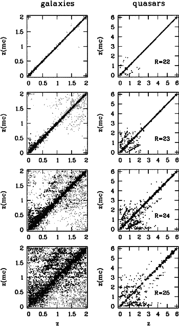
 )
among simulated galaxies with R=23 in setup A separated for quiescent and starburst
objects. The solid line shows results for the Minimum Error Variance estimators (MEV
and MEV+ are virtually the same) and the grey line those for the Maximum Likelihood
estimator (ML). Starburst systems show higher errors and some large mistakes with
)
among simulated galaxies with R=23 in setup A separated for quiescent and starburst
objects. The solid line shows results for the Minimum Error Variance estimators (MEV
and MEV+ are virtually the same) and the grey line those for the Maximum Likelihood
estimator (ML). Starburst systems show higher errors and some large mistakes with