3 The classification libraries

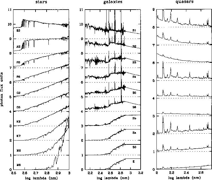
Figure 1: This diagram shows a few selected spectra from our template libraries. The shown wavelength scale runs from 315nm to 1000nm for stars (left), from 125nm to 1600nm for galaxies (center) and from 100nm to 550nm for quasars (right). The flux is $\lambda f_\lambda$ in units of photons per nm, time intervall and sensitive area and offset by one unit per step within a class. The flux scale is normalised to unity at 800nm for stars, arbitrary for galaxies, and normalised to 0.2 at 250nm for quasars. The stellar templates are taken from Pickles (1998), the galaxy templates from Kinney et al. (1996) and quasar templates are modelled after Francis et al. (1991). The quasar diagram shows nine spectra with three different spectral indices (-2.0, -0.6, +0.8) and three different relative emission-line intensities (0.6, 2.1, 5.7)

We assembled the color libraries from intrinsic object spectra assuming no galactic reddening. Clearly these libraries can only be sufficient when observing fields with low extinction and little reddening. Usually, such fields are chosen for deep extragalactic surveys and the CADIS fields in paticular were carefully selected to show virtually no IRAS 100$\mu$ flux (below 2MJy/sterad), so we expect "zero'' extinction and reddening there. When applying this color classification to fields with reddening, the libraries would have to be changed accordingly.

Obviously, the libraries should contain a representative variety of objects, but still they can never be assumed to cover a complete class including all imaginable oddities. When classes are enlarged to cover as many odd members as possible, there is a trade-off to be expected between classifying the odd ones right, and introducing more spatial overlap between the classes in general, i.e. introducing more confusion among normal objects. The spectral libraries we employ are partly based on observations only and partly mixed with model assumptions. Our particular choice of libraries is founded on experience we gained within the CADIS survey, where we found several other published templates to be less useful.

3.1 The star library

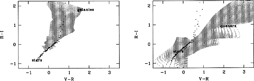
For the stars, we picked the spectral atlas of Pickles (1998), that contains 131 stars with spectral types ranging from O5 to M8. It covers different luminosity classes but concentrates on main sequence stars, and it also contains some spectra for particularly rich metallicities. For the surveys in consideration, very young and very luminous stars should not be expected, but we include the entire library nevertheless (see Fig.1). Stars later than M8 are missing in the library, but they do show up in deep surveys like CADIS (Wolf et al. 1998). These objects are interesting on their own, of course, but they are so rare, that a couple of misclassifications do not hurt the statistics on other objects.

In earlier stages of the CADIS survey, we reported using the Gunn & Stryker (1983) atlas of stellar spectra (see e.g. Wolf et al. 1999), which has a number of disadvantages compared to the new work by Pickles. Our impression is that the Pickles spectra have a better calibration in the far-red wavelength range and are less affected by noise there. Especially, broad absorption troughs in M stars are rendered more accurately in the Pickles templates, which can be quite relevant for medium-band surveys. Also, they cover the NIR region and, e.g., the entire CADIS filter set all the way out to the $K^\prime$ band, thereby omitting the need for homemade extrapolations. Since it contains two different metallicity regimes, it covers the range of possible stellar medium-band colors better than the Gunn & Stryker atlas, most notably among M stars for colors sensitive to their deep absorption features and, e.g., among K stars for colors probing the Mg I absorption.

The atlas is not structured as a regular grid in the stellar parameters and we consider the resulting color library an unsorted set without internal structure. If variations in dust reddening are to be expected within the field as in the case of Galactic stellar observations, this effect should be treated as an additional parameter in the library.

For multi-color surveys aiming specifically at Galactic stars, one would ideally like to have a library organized as a regular grid in effective temperature, surface gravity and metallicity, which could, e.g., be derived from model atmospheres. Such a fine classification is not needed for extragalactic surveys, where the focus is on galaxies and quasars. We gained some experience with the stellar spectra from the model grid by Allard (1996), but we decided not to use it, since the overall colors seemed to be better matched by the Pickles library.

3.2 The galaxy library

The galaxy library is based on the template spectra by Kinney et al. (1996). These are ten SEDs averaged from integrated spectra of local galaxies ranging in wavelength from 125 nm to 1000 nm. The input spectra of quiescent galaxies were sorted by morphology beforehand to result in four templates called E, S0, Sa and Sb. The starburst galaxies were sorted by color into six groups yielding six more templates called SB6 to SB1. Based on the observation, that color and morphology of galaxies correlate, this template design seems reasonable. This way the classification can indirectly measure morphology of galaxies via their SED, at least as far as the locally determined color-morphology relation holds at higher redshift.

The templates contain a very deep unidentified absorption feature around 540 nm, which we supposed to be an artifact of the data reduction and eliminated. We left the abundant structures in the UV unchanged, although some of them might be noise and we do not know how to interprete them. We modelled a near-infrared addition heuristically by a simple law consistent with the $I-K^\prime$-colors of a sample of galaxies with known spectroscopic redshifts (see Paper II). Using this addition, we extended the spectra out to 2500 nm, and actually replaced the spectrum starting from 800 nm to eliminate the noise in the templates redwards of 800 nm (see Fig.1). Quiescent galaxies were extended according to $f_\nu \sim \nu^{-1}$, while starburst galaxies seemed most consistent with an extension of $f_\nu \sim \nu^{-1/3}$.

We consider the templates to form a one-dimensional SED axis of increasingly blue galaxies and fill in more templates to obtain a dense grid of 100 SEDs. Our interpolation is done linearly in color space, and the number of filled-in SEDs is chosen such, that the color space is filled rather uniformly. The new SEDs are denominated as numbers from 0 to 99, where the ten original SEDs used for the interpolation reside at the following numbers:

E - S0 - Sa - Sb - S6 - S5 - S4 - S3 - S2 - S1

0 - 15 - 30 - 45 - 75 - 80 - 85 - 90 - 95 - 99.

Internal reddening is considered an important effect for the colors of galaxies and especially common among later types. While trying to account for it, we realized that its effect is merely one of shifting the zeropoint in the SED and hardly one of changing the redshift estimates. If we did introduce an independent reddening parameter, it would be almost colinear with the SED axis itself. Therefore, we opted for using the templates as determined from real galaxies and provided by Kinney et al. (1996), since they probably contain already a typical distribution of reddened objects. Due to our scheme of SED interpolation, we can still classify galaxies, which are reddened more or less than usual.

We also tried to change the SED interpolation scheme by relocating the templates to different SED numbers, which did not seem to improve the results. The color library was calculated for 201 redshifts ranging in steps of $\Delta z = 0.01$ from z=0 to z=2, finally containing $201 \times 100$ members. We did not intend to go beyond a redshift of 2, since our survey applications have typically not become deep enough, yet, to see such objects in useful numbers.

The main shortcoming of this library is that the 1-dimensional SED allows no variation in emission-line ratios independent of the global galaxy color. Since medium-band filters can contain strong emission-line signals from faint galaxies, an observed emission-line ratio detected by two suitably located filters can be in disagreement with the global SED traced by all other filters. Since especially the CADIS filters are placed to deliver multiple detections of emission lines at several selected redshifts, some degradation in real performance could be expected with respect to the simulation (see Paper II).

3.3 The quasar library

The quasar library is designed as a three-component model: We add a power-law continuum with an emission-line contour based on the template spectrum by Francis et al. (1991), and then apply a throughput function accounting for absorption bluewards of the Lyman-$\alpha$ line. We modeled a throughput function T₀ after visually inspecting spectra of $z\approx 4$-quasars published by Storrie-Lombardi et al. (1996), and keep its shape constant (see Fig.3) while varying its scale to follow the increasing continuum depression $D_{\rm A}$ towards high redshift. Using data from Kennefick (1996) and Storrie-Lombardi et al. (1996) as a guideline, we arrived at

T (z) = T₀^(z/4.25)2 . (28)

The intensity of the emission-line contour was varied only globally, i.e. with no intensity dispersion among the lines. As long as typically only one medium-band filter is brightened by a prominent emission line, the missing dispersion should not affect the classification (see Fig.2). For the intensity factor relative to the template, $e^\epsilon$, ten values were adopted ranging in steps of $\Delta \epsilon = 0.25$ from $\epsilon = -0.5$ to $\epsilon = 1.75$ on a logarithmic scale, which is roughly 0.6 times to 5.7 times the template intensity. Originally, we tried a range from 0.3 times to 2.7 times, but the first twenty quasars found in CADIS contained mostly strong lines, which are better represented by the current limits.

The slope of the power-law continuum $f_\nu \sim \nu^\alpha$ was varied in 15 steps of $\Delta \alpha = 0.2$ ranging from $\alpha = -2.0$ to $\alpha = 0.8$. The library was calculated for 301 redshifts ranging in steps of $\Delta z = 0.02$ from z=0 to z=6, finally containing $301 \times 15 \times 10 = 45\,150$ members. As a future improvement one could imagine the inclusion of Seyfert I galaxies with nuclei of rather low luminosity, i.e. spectra coadded as a superposition of a host galaxy spectrum with a broad-line spectrum for the nucleus.

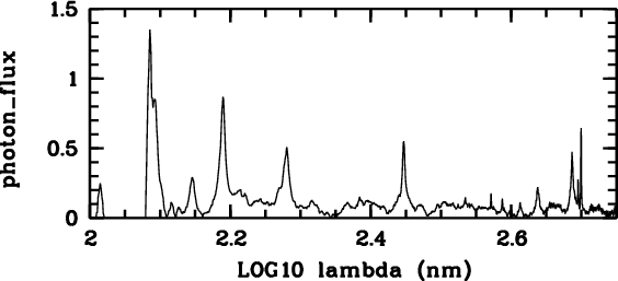Figure 2: The quasar library is based on an emission line contour taken from the quasar template spectrum by Francis et al. (1991). The wavelength scale runs from 100nm to 550nm and the flux is $\lambda f_\lambda$ in units of photons per nm, time intervall and sensitive area (arbitrary units)

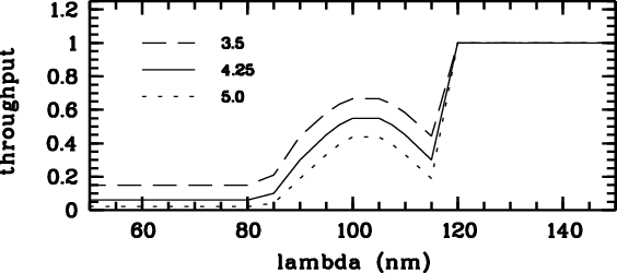Figure 3: For the quasars we assumed a throughput function for the Lyman-$\alpha$forest which we derived from a visual inspection of quasar spectra published by Storrie-Lombardi et al. (1996). The scale of this function depends on redshift and is shown for z=3.5, 4.25 and 5.0

3.4 Calculation of color libraries

As a first step, the spectral libraries were transformed into color index libraries representing precisely the set of filters and instruments in use. The use of precalculated filter measurements rather than fully resolved flux spectra removes any computationally expensive calculations for synthetic photometry from the process of classifying the object list. The use of color indices omits the needs for any flux normalisation, further speeding up the classification. A list of $\sim$10⁴ objects and $\sim$10 colors can be classified within a couple of hours on a SUN Enterprise II workstation even when using $\sim$10⁵ templates.

For best results it is required that the color libraries are calculated for an instrumental setup resembling precisely the observed one, i.e. the synthetic photometry calculation has to take every dispersive effect into account. We decided to use photon flux colors derived from the observable object fluxes, averaged over the total system efficiency of each filter and assuming an average atmospheric extinction.

Figure 4: These diagrams of B-V vs. R-I color show the class models of stars (black) and galaxies (grey) on the left, and stars (black) and quasars (grey) on the right to illustrate their location in color space. The colors plotted are photon flux color indices, which are offset compared to astronomical magnitudes, such that Vega has V-R= -0.41 and R-I= -0.61

The shape of the filter transmission curves needs to be known precisely, and is in the best case measured within the imaging instrument itself under conditions identical to the real imaging application. This is easily possible with, e.g., the Calar Alto Faint Object Spectrograph (CAFOS) at the 2.2 m telescope on Calar Alto, Spain: in this instrument light from an internal continuum source is sent first through the filterwheel and second through the grism wheel before reaching the detector. Images are taken with and without the filter, so their ratio gives immmediately the transmission curve. Colors measured in narrow filters depend sensitively on the transmission curve, whenever strong spectral features are probed, e.g. the continuum drop at the Ca H/K absorption or the Mg I absorption in late-type stars. In these cases the curve needs to be known rather precisely, since otherwise the calibration would be off, and misclassifications could occur.

3.5 Potential improvements on the classification

The quality of the classification reached depends on just the three elements of the method: the quality of the measured data, the choice of the classifier and the quality of the libraries forming the knowledge database for the comparison. In principle, improvements on the performance can be achieved only in the following respects:

• improvements on the data: the filter set could be changed and potentially be tailored to a specific goal of the survey; the exposure time could be increased or distributed better among the individual filters; the accuracy of the calibration could be increased;

• improvements on the classifier: the classifier can not be improved fundamentally. A very crucial ingredient for a statistically correct result is a valid assessment of the measurement errors since they form a basic input to the probability calculation. Some simplifications have been introduced which make a difference only among faint objects which are hardly classifiable anyway. For specific goals the classifier can be modified accordingly, and diverse goals potentially ask for contrary strategies. A global maximum in the classification reliability is best achieved by weighting rare classes lower, while searching for rare objects would profit from weighting them higher.

• improvements on the libraries: this is the most important aspect, since any library-based classifier can obviously recover identifications only if they are contained in the library, and if their spectral profile is well-known. Altogether, this work has strongly benefitted from templates and libraries published in the literature (Francis et al. 1991; Kinney et al. 1996; Pickles 1998), which we could arrange into an ordered database. Their limitations are discussed in the respective section. Our present experience suggests that empirical spectra work better for our survey data than purely theoretical spectra. In the future, we would also like to check some of our model assumptions used in the libraries against observations.