Generally speaking, classification is a process of pattern recognition which usually has to deal with noisy data. Mathematically, a classifier is a function, which is mapping a feature vector of a measured object characteristics onto a discriminant vector, that contains the object's likelihoods for belonging to the different available classes. Any classification relies on the feature space being chosen such that different classes cover different volumes and overlap as little as possible to avoid ambiguities.
If a survey is designed without class definitions in mind, it will be difficult to choose a set of measurable features for a tailored classification. Also, only unsupervised classifiers (= working without knowledge input) can be used to work on measured object lists. In this case, a classifier can find distinguishable classes, e.g. by cluster analysis. This process leads to a definition of new class terms which depends strongly on the visible features taken in account.
For any classification problem, it is of great advantage, if class terms are defined a priori and encyclopedic knowledge is available about measurable features and their typical values. Then models of the classes representing this knowledge can be constructed to serve as an essential input to a supervised classifier (= using input knowledge as a guide). When selecting the features, two potential problems should be avoided: One is the use of well-known but hardly discriminating features, which will obviously not improve the classification but just increase the effort. The other is using features which are not well-known and therefore can easily cause mistakes in the classification. Especially, with high measurement accuracy this can lead to apparent unclassifiability when an object looks different than expected.
Two different types of class models can be distinguished depending on the uniqueness of the classification answer:
While classes are discrete entities, a statistical classification can also work on continuous parameters. The discriminant vector then becomes a likelihood function of the parameter value. Based on this distinction classification problems can be considered as decision problems for discrete variables and estimation problems for continuous variables (Melsa & Cohen 1978a). In either case, a definite statistical classification containes two consecutive steps: First, the discriminant vector is determined (see Sect. 2.2) and second, it is mapped either by decision to a final class or to a parameter estimate (see Sect. 2.3).
We assume an object with m features being measured by any device, thus displaying
the feature vector
 .
We consider n classes
.
We consider n classes
 as a possible nominal interpretation and denote the likelihood of this object to
belong to the class ci as
as a possible nominal interpretation and denote the likelihood of this object to
belong to the class ci as
 .
A true member of class ci has an
a priori probability of displaying the features
.
A true member of class ci has an
a priori probability of displaying the features  given by
 .
.
Initially, we assume a simple case of uniquely defined class models, where all
members of a single class ci have the same intrinsic features
 ,
so
that any spread in measured
values arises solely from measurement errors.
Assuming a Gaussian error distribution for every single feature, it follows
(Melsa & Cohen 1978b), that
,
so
that any spread in measured
values arises solely from measurement errors.
Assuming a Gaussian error distribution for every single feature, it follows
(Melsa & Cohen 1978b), that
 |
(1) |
where
 is the measurement error in case the object does belong
to ci and
is the measurement error in case the object does belong
to ci and
 is its transposed version. Each feature qkis measured with its own error variance
 ,
which are the diagonal elements
in the variance-covariance matrix V. If all the features are statistically
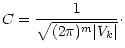
independent, the off-diagonal elements vanish. The normalisation factor C is
,
which are the diagonal elements
in the variance-covariance matrix V. If all the features are statistically
independent, the off-diagonal elements vanish. The normalisation factor C is
 |
(2) |
As contained in the discriminant vector, the likelihood for an object observed with
to belong to class ci is then
However, in realistic cases the classes themselves are extended in feature space and
their volume might have rather complicated shapes. In the spirit of Parzen's kernel
estimator (Parzen 1963) the extended class ci can be represented by a dense cloud
of individual uniquely defined (point shape) members cij. Every member accounts
for some a-priori probability to display ,
given as
 ,
just
as if it were a "class'' on its own. The complete class ci is now rendered as a
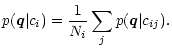
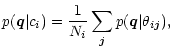
superposition of its Ni members and adds up to a total probability of
,
just
as if it were a "class'' on its own. The complete class ci is now rendered as a
superposition of its Ni members and adds up to a total probability of
In an estimation problem the probability functions have the same form, except
for changes in the notion:  denotes the parameter to be estimated, and
ideally the class model ci had a continuous shape covering the range of expected
values. The discriminant vector would then be a function
denotes the parameter to be estimated, and
ideally the class model ci had a continuous shape covering the range of expected
values. The discriminant vector would then be a function
 .
Again,
the class model can be approximated by a discrete set of members sampling the
range of interest at sufficient density.
.
Again,
the class model can be approximated by a discrete set of members sampling the
range of interest at sufficient density.
The astronomical application discussed in this paper poses a mixture of decision and
estimation problems which can be realized simultaneously with a unified approach:
the
decision may choose from the three classes c1 = stars, c2 = galaxies and c3
= quasars, and an estimation process takes care of the parameters redshift and
different spectral energy distributions (SED). The internal structure of every class
ci is then spanned by its individual parameter set
 ,
either following a grid design or being unsorted if no
parameter structure is needed.
,
either following a grid design or being unsorted if no
parameter structure is needed.
If one chooses to approximate the spatial extension of a class by a dense grid
sampling discrete parameter values, two problems are solved at once: on the one hand,
an internal structure is present for estimating parameters, and on the other hand,
the class is well represented for calculating its total probability
.
Altogether, the probability function with internal parameters
 being resembled by class members
 is then
 |
(5) |
with the total probability for class ci being
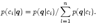
and the equation for the class likelihood function still being
 |
(7) |
Based on these probability functions the classification can perform a decision between object classes and estimations of redshift and other object parameters at once. Two different analyses are integrated into one paradigm and calculated efficiently by evaluating the same probability density function.
Decision rules are functions mapping a discriminant vector
 to a
decision value d. The value di denotes a decision in favor of class ci, i.e.
the object displaying features
is then assumed to belong to this class. The
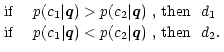
most simple decision rule is the maximum likelihood (ML) scheme, which decides for
the one class with the highest likelihood p. In case of two classes existing this
means
to a
decision value d. The value di denotes a decision in favor of class ci, i.e.
the object displaying features
is then assumed to belong to this class. The
most simple decision rule is the maximum likelihood (ML) scheme, which decides for
the one class with the highest likelihood p. In case of two classes existing this
means
 |
(8) |
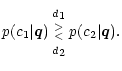
A more compact notion for the same rule is
 |
(9) |
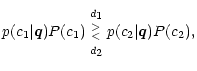
Depending on the purpose of the classification tailored improvements can be made to
this rule. The probability of error (PoE) method, e.g., attempts to minimize the rate
of misclassifications by including the a-priori-probability for observing a member of
a given class. Following Bayes theorem these "priors'', denoted P(c1) and
P(c2), are just the relative abundance of the class in the whole sample. The PoE
decision rule is then
 |
(10) |
which causes somewhat ambiguous objects to be preferentially classified as belonging
to the more common class. Rare objects are then less likely to be found at all, but
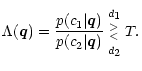
the overall performance of the classifier improves. A general approach uses any type
of priors for trimming the classification towards specific goals, so every decision
rule compares the likelihood ratio  with a threshold T and follows the
form (with T=1 for ML decision)
with a threshold T and follows the
form (with T=1 for ML decision)
 |
(11) |
Estimation rules are functions mapping a discriminant vector
 to an estimated value
 .
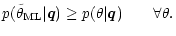
The most simple estimation rule is again the
maximum likelihood (ML) rule, which chooses the one parameter value with the highest
likelihood p, i.e., the ML estimator is given by
.
The most simple estimation rule is again the
maximum likelihood (ML) rule, which chooses the one parameter value with the highest
likelihood p, i.e., the ML estimator is given by
 |
(12) |
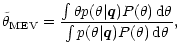
The Bayesian approach can also be applied to continuous variables, whereas one
special case is of particular interest: if the error distribution of the feature
measurement is Gaussian, and if the goal is to minimize the variance of the true
estimation error, then the optimum estimation rule can be derived analytically
(Melsa & Cohen 1978b). This minimum error variance (MEV) estimator is given by
 |
(13) |
and it is equivalent to interpreting the discriminant vector as a statistical
ensemble and determining the mean of the distribution. It is also dubbed mean square
estimator or conditional mean estimator. Note that, if
is
symmetric in
and unimodal, the MEV estimator is identical to the ML
estimator.
Deep extragalactic surveys usually contain mostly galaxies, fewer stars and a tiny
fraction of quasars, with relative numbers on the order of 100:10:1. A survey at
galactic latitudes above
 with a limiting magnitude of R=23and an area of 1
 ,
e.g., should contain roughly 30000 galaxies
(Metcalfe et al. 1995), some 3000 to 6000 stars (Bahcall & Soneira 1981;
Phleps et al. 2000), and about 400 quasars
including Seyfert-1 galaxies (Hartwick & Schade 1990). Any classification would ideally be capable
of distinguishing all three classes of objects. Only in surveys, which do not care
about the rare quasars, their class could be dropped and the classification needed to
separate only stars from galaxies.
,
e.g., should contain roughly 30000 galaxies
(Metcalfe et al. 1995), some 3000 to 6000 stars (Bahcall & Soneira 1981;
Phleps et al. 2000), and about 400 quasars
including Seyfert-1 galaxies (Hartwick & Schade 1990). Any classification would ideally be capable
of distinguishing all three classes of objects. Only in surveys, which do not care
about the rare quasars, their class could be dropped and the classification needed to
separate only stars from galaxies.
In addition to the class itself, plenty of physical parameters could potentially be recovered from an object's photometric spectrum. Most importantly, we would like to determine redshift estimates for galaxies and quasars. In addition, the spectral energy distribution of galaxies contains information about their star formation rate and the age of their stellar populations. A photometric spectrum of sufficiently high spectral resolution can even allow to estimate the intensity of emission-lines. Finally, the spectra of stars tell mostly their effective temperature, but also their metallicity and their surface gravity.
The literature provides abundant knowledge of spectral properties for all three object classes. Synthetic photometry can use published spectra together with efficiency curves from the survey filter set in order to obtain predicted colors of objects. Sometimes, model assumptions are needed to fill in data gaps present in the literature, which could either be gaps on the spectral wavelength axis or gaps on physical parameter ranges, e.g. star-formation rate. Eventually, systematic multi-color class models can be calculated from published libraries covering various physical parameters. These can serve for later comparison with observed data. Therefore, we decided to build a statistical classification based on published spectral libraries and a limited number of model assumptions (see Sect.3).
In a multi-color survey the dominant information gathered are the object fluxes in the different filters. We decided to use the color indices as an input to the classification rather than the fluxes themselves, which eliminates one dimension from the problem by omitting the need for any flux normalisation, that remains as an additional fit parameter in template fitting procedures. It will be shown in Sect.2.5, that the color-based approach is equivalent to the flux-based one under certain constraints.
Morphological information is typically also available to some extent and can be included in the classification based on the assumption that only galaxies are capable of showing spatial extent. But this should be done carefully, since luminous host galaxies can render quasars as extended. Also, if the image quality varies across the observed field, the morphological analysis is of limited use for not clearly extended sources.
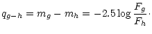
We define the color qg-h as a magnitude difference between the flux measurements
in two filters Fg and Fh:
 |
(14) |
Obviously, the color system depends on the filter set chosen and also on the flux
normalisation used. As long as the flux errors are relatively small, the linear
approximation of the logarithm can be used to express magnitude errors as
 ,
so that the error of the color is
,
so that the error of the color is
 |
(15) |
Since the likelihoods determined for the classification depend sensitively on the
colors
and their errors
 ,
both values must be carefully
calibrated. If any color offset is present between measurement and model, the
classification will go wrong systematically. If errors are underestimated, the
likelihood function could focus on a wrong interpretation, rather than including the
full range of likely ones. Overestimated errors will obviously diffuse the
likelihoods and give away focus which is originally present in the data. The
approximation of errors as presented will only work well with flux detections of at
least 5
,
both values must be carefully
calibrated. If any color offset is present between measurement and model, the
classification will go wrong systematically. If errors are underestimated, the
likelihood function could focus on a wrong interpretation, rather than including the
full range of likely ones. Overestimated errors will obviously diffuse the
likelihoods and give away focus which is originally present in the data. The
approximation of errors as presented will only work well with flux detections of at
least 5 to 10,
but at lower levels the classification is likely to
fail anyway, so we ignore this concern.
to 10,
but at lower levels the classification is likely to
fail anyway, so we ignore this concern.
Given
and
a measured object is represented by a Gaussian
error distribution rather than a single color vector. If colors are measured very
accurately and the object is rendered as a narrow distribution, it could possibly
fall between two grid steps of a discrete class model and "get lost'' for the
classification. In this case low likelihoods would be derived despite the spatial
proximity of object and model in terms of metric distance. The likelihood function
would appear not much different from that of a truely strange object residing off the
class in an otherwise empty region of color space. In technical terms, the
classification would violate the sampling theorem (Jähne
1991), and the
probability functions would not be invertible any more.
For discrete class models the sampling theorem requires that every measurement falling inside the volume of a model should "see'' at least two model members inside of its Gaussian core. Due to practical limitations of computing time and storage space, it does not make sense to develop discrete models with virtually infinite density accounting for arbitrarily sharp measurements. Also, for measurements with low photon noise the dominant source of error will be the limited accuracy of the color calibration.
The solution to the problem is then to design the discrete model with the achievable measurement accuracy in mind, and to smooth the discrete model into a continuous entity by convolving its grid with a continuous function that is wide enough to prevent residual low-density holes between the grid points. A sensible smoothing width would just fulfill the sampling theorem, i.e. the smoothing function should roughly stretch over a couple of discrete points. As a result, even an extremely sharp measurement will be covered by the model and classified correctly.
Higher resolution would only increase the computational efforts while lower resolution would ignore information which is present in the data and therefore potentially worsen the classification. From a different point of view, one could leave the discrete model unchanged and claim the data to have larger effective errors by including the calibration errors thereby limiting the width of the Gaussian data representation to a lower threshold, which will always ensure the sampling theorem on the discrete grid anyway.
Both approaches are mathematically identical, if one chooses to represent the
calibration errors as well as the smoothing function by a Gaussian. Due to the
symmetry of the Gaussian function, convolving the discrete grid or convolving the
error distribution of the data yields the same result. The choice of the Gaussian is
computationally very efficient, because the convolution of the Gaussian measurement
with the Gaussian calibration error results in another Gaussian of enlarged width. As
mentioned in Sect.5.1 and discussed in Paper II, a survey in the
visual bands can be calibrated with a relative accuracy on the order of 3% between
the different filters. Therefore, we decide to apply a
 -Gaussian as a
smoothing function.
-Gaussian as a
smoothing function.
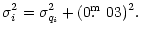
In summary, we apply the formalism presented in Sect. 2.2 in the
following way: the errors
 of the colors qi are convolved with the
smoothing
-Gaussian and as a result the effective errors are
of the colors qi are convolved with the
smoothing
-Gaussian and as a result the effective errors are
 |
(16) |
For simplicity, we assume the individual colors to be uncorrelated, which is actually
not true for filters sharing spectral regions in their transmission. The
variance-covariance matrix then becomes diagonal
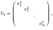 |
(17) |
and the probability function turns into
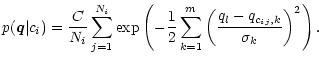 |
(18) |
Based on the three object classes discussed the likelihood function is
 |
(19) |
Considering three classes implies that extremely faint objects with large errors get
average probabilities of 33% assigned for all classes. In general applications, we
use a decision rule for an object seen as ,
which requires that one class is
at least three times more probable than the other two classes put together, i.e.:
If there is one class with, then we assign this class to the object, but if all classes have likelihoods below 0.75, we call it unclassifiable.
For the detection of unusual objects, we look at the color distance of an object to
the nearest member of any class model to derive a statistical consistency with the
class. The value of this consistency depends on the different color variances and can
be calculated from  -statistics. Lacking an analytic expression we use
-tables (Abramowitz & Stegun 1972) to evaluate the statistical consistency between class and
object. In practice, the resulting -values need to be normalised to a
plausible scale, since the raw values obtained are enlarged artificially due to the
discrete sampling of the library and cosmic variance. We use the following operative
criterion for the selection of unusual objects:
-statistics. Lacking an analytic expression we use
-tables (Abramowitz & Stegun 1972) to evaluate the statistical consistency between class and
object. In practice, the resulting -values need to be normalised to a
plausible scale, since the raw values obtained are enlarged artificially due to the
discrete sampling of the library and cosmic variance. We use the following operative
criterion for the selection of unusual objects:
If an object is inconsistent at least at a confidence level of 99.73% (i.e. 3
Strange objects can formally be classifiable, if the likelihoods still prefer a certain class membership. They have either intrinsically different spectra without counterparts in the class models, or they are reduction artifacts, e.g. when neighboring objects affect their color determination, and this is not taken into proper account for the error calculation.
Apart from the rather trivial ML estimator, we use the MEV estimator to obtain
redshifts and SED parameters of galaxies and quasars. Their class models are designed
as regular grids (see Sect.3) with members cij residing at redshift zij.
The MEV estimator for the redshift is then
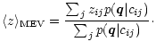 |
(20) |
It is applied to the class models for galaxies and quasars independently and for each
class interpretation an independent redshift estimate is obtained. There is also an
assessment for the likely error of the z estimate given by the variance of the
distribution
 :
:
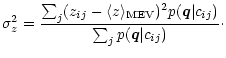 |
(21) |
This estimation scheme would be sufficient, if models had a rather simple shape in
color space, i.e. if color space and model parameter space could easily be mapped
onto each other. In fact, the class model for galaxies and particularly the one for
quasars can have very complicated folded shapes in color space, so that the
distribution
can have a correspondingly complicated structure that is
not at all well described by mean and variance.
Therefore, we distinguish three cases: unimodal (single peaked), bimodal (double
peaked) and broad distributions. In unimodal cases
 and
and
 are appropriate reductions of
.
In bimodal cases we split the
redshift axis in two intervals delimited at
and obtain two
alternative unimodal solutions with relative probabilities given by the p sums in
the two intervals. If the distribution is so broad, that it starts to resemble a
uniform distribution,
approaches the mean z value of the
model and
approaches
are appropriate reductions of
.
In bimodal cases we split the
redshift axis in two intervals delimited at
and obtain two
alternative unimodal solutions with relative probabilities given by the p sums in
the two intervals. If the distribution is so broad, that it starts to resemble a
uniform distribution,
approaches the mean z value of the
model and
approaches
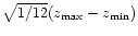 .
In order to keep our
statistics clean from such mean redshift contaminants, we cut off the estimator at
some uncertainty:
.
In order to keep our
statistics clean from such mean redshift contaminants, we cut off the estimator at
some uncertainty:
If an object has, then we ignore the MEV estimate and call its redshift uncertain.
In particular, it is possible, that an object has a bimodal distribution with one peak (result) and one broad (uncertain) component. In the following, we denote this extended scheme of MEV estimates accounting for possible bimodalities as our MEV+ estimate. In Sect.4.4 we will compare the performance of all three estimators, ML versus MEV and MEV+.
An effort was made to implement a classification code optimized for short computing
time. The use of precalculated class models eliminates any synthetic photometry from
a typical fitting procedure. Furthermore, the use of colors instead of fluxes
eliminates the need for finding a flux normalisation. In terms of CPU time, the
classification of one object contains mainly the calculation of the probability
for every class member, which involves first adding up all
 -scaled squared color differences and second evaluating an exponential
function of the resulting sum that is already a measure of strangeness. Summing up
the
to obtain class likelihoods and deriving mean and variance of
the internal class parameters should take less time than calculating the probability
density function, if more then ten color axes are taken into account. With class
models containing about 50000 members and 13 colors, the full classification of one
object takes about 0.3sec when running on a 200MHz Ultra Sparc CPU inside a SUN
workstation. Since different survey applications might require different sample
selection schemes, we decided to calculate and store discriminant vectors for all
objects and select subcatalogs for further analysis later.
-scaled squared color differences and second evaluating an exponential
function of the resulting sum that is already a measure of strangeness. Summing up
the
to obtain class likelihoods and deriving mean and variance of
the internal class parameters should take less time than calculating the probability
density function, if more then ten color axes are taken into account. With class
models containing about 50000 members and 13 colors, the full classification of one
object takes about 0.3sec when running on a 200MHz Ultra Sparc CPU inside a SUN
workstation. Since different survey applications might require different sample
selection schemes, we decided to calculate and store discriminant vectors for all
objects and select subcatalogs for further analysis later.
We now show, that the color-based classification yields the same best fit as a flux
based template fitting algorithm. Lanzetta et al. (1996), e.g., calculate a
likelihood function depending on redshift z, a spectral energy distribution and a
flux normalisation parameter A, following the form:
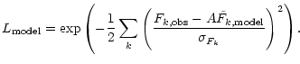 |
(22) |
Basically, the likelihood determination relies on the squared photometric distance
d between observation and model, resulting from the flux differences
 in each filter:
In the color based approach there are n-1 color indices contributing distance components and we assume the single constraint, that there is one particular base filter approximately free of flux errors, e.g. a deeply exposed broad-band filter. The color indices are made by comparing any filter to this base filter ensuring optimum errors for the colors. In this scheme, any errors in the relative calibration are absorbed into the color indices. Therefore, it is very important, that the base filter is not wrongly calibrated with respect to the other wavebands, since the error would spread into the entire vector of color indices.
We then look only at a range of good fits, and do not mind rather crude
 -approximations for relatively bad fits which are anyway ruled out as
solutions. Also, we consider only measurements with
-approximations for relatively bad fits which are anyway ruled out as
solutions. Also, we consider only measurements with
 ,
which allows the assumption of Gaussian color errors and a linear approximation of
the logarithm. The distance components are:
,
which allows the assumption of Gaussian color errors and a linear approximation of
the logarithm. The distance components are:
 |
= | 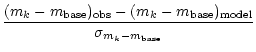 |
|
| = |  |
(24) |
Using the terms
and
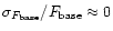 ,
we obtain
,
we obtain
 | |||
 |
(25) | ||
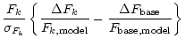
Expanding the logarithm for
 ,
we get
,
we get
|
 |
 |
|
|
 |
(26) |
The first term is typically on the order of 1, while the second term is on the order
of
 and the third one of
 .
Therefore, the last two terms can be dropped and the expression for
.
Therefore, the last two terms can be dropped and the expression for  reduces to
 |
(27) |
which is identical to the expression used in the flux template fitting method shown in Eq. (23).
In the previous section, we had discussed the relevance of a common base filter for the various color indices, which is supposed to have relatively small flux errors in order to keep the color errors as low as possible. Our multiband survey applications usually involve a smaller number of broad bands as well as a larger number of medium-band observations. For these, we decided to form color indices from broad bands neigboring on the wavelength axis, i.e. U-B, B-V, V-R and R-I, which we assume to be the optimum solution for comparably deep bands. Each of the shallower medium bands we combine with the most nearby broad-band in terms of wavelength, which then serves as a base filter for the medium-band color indices, e.g. B-486 or 605-R, where letters denote broad bands and numbers represent the central wavelength of medium-band filters measured in nanometers.
In terms of flux template fitting, this scheme of color indices means, that we use a
few deep broad bands to fit the global shape of the SED, and then use a few groups of
medium bands around each deep broad-band to fit the smaller-scale shape locally. The
-values of the global fit and the several local fits are then just added up
to the total .
This scheme has a particular advantage over a solely global
flux fitting: the local fits can well trace spectral structures, even if the global
distribution of the object differs from the template (e.g. as it could be caused by
extinction). Therefore, it is not too dependent on accurate global template shapes
and it can use the ability of the medium bands to discriminate narrow spectral
features for a more accurate classification. Of course, this advantage vanishes
immediately for a pure broad-band survey, where local structures in the spectrum are
not traced, and therefore no local fits are available for the -sum.
Copyright ESO 2001