A&A 405, 1177-1189 (2003)
DOI: 10.1051/0004-6361:20030653

Efficient first-order performance estimation for high-order adaptive optics systems

R. C. Flicker

Lund Observatory, Box 43, 22100 Lund, Sweden

Received 3 February 2003 / Accepted 25 April 2003

Abstract
It is shown how first-order performance estimation of high-order adaptive optics (AO) systems may be efficiently implemented in a hybrid numerical simulation by the use of 1) sparse matrix techniques for wavefront reconstruction, 2) undersampled pupil-plane turbulence-induced aberrations, and 3) analytical models that compensate - in the limit of infinite exposure time - for the errors introduced by undersampling. A sparse preconditioned conjugate gradient (PCG) method is applied for wavefront reconstruction, and it is seen that acceptable AO performance may be achieved at a relative error tolerance of 0.01, at which the computational cost of the sparse PCG scales approximately as  O(n^1.2), where n is the number of actuators in the system. Estimations of adaptive optics performance for extremely high-order systems are presented, including multi-conjugate and laser-guide-star-based systems. The scaling laws for AO performance with telescope diameter D and turbulence outer scale L₀ coupled with the use of laser guide stars are also investigated. It is shown that a single or a small number of laser guide stars (LGS) may still provide a useful level of compensation to telescopes with diameters in the range 30-100 m, if L₀ is on the order of or smaller than D. The deviations from Kolmogorov theory are also investigated for LGS AO. To the best of the author's knowledge, results presented for a n=65 282 case represent the largest multi-conjugate adaptive optics system simulated in full to date.

Key words: instrumentation - adaptive optics - methods - numerical

1 Introduction

The technology of adaptive optics (AO) is attaining an increasingly more prominent role in ground-based optical astronomy as the next generation of telescopes and instrumentation is being planned. It is clear (Ragazzoni et al. 2000; Snel & Ardeberg 2002; Hawarden et al. 2002; Gilmozzi 2000) that a near-diffraction-limited mode of imaging will be required of future ground-based telescopes with aperture diameters ranging upward from tens of meters to $\sim$100 m, in order to enable such science as will be unique to that large a telescope and thereby justify the staggering costs involved. AO systems, as generically outlined in Fig. 1, are thus moving toward becoming an integral part of a telescope, and may rightfully claim to be one of the important "raisons d'être'' for future extremely large telescopes (ELTs). It can be problematic, however, to study and design adaptive optics systems when the required order of the system, as represented henceforth by the total number of actuators n, becomes very large. The computational cost for a conventional wavefront reconstruction algorithm, a simple matrix-vector multiplication, is of the order O(n²) floating point operations and the cost for the matrix inversion required to prepare the estimator scales as O(n³). Since n scales linearly with the surface area of the telescope aperture, the computational costs for these two actions will scale as O(D⁴) and O(D⁶), where D is the diameter of the telescope. Hence it is clear that, at some point, a practical problem will arise both in simulation and real-time control of the system as D grows large. These scaling laws are illustrated in numbers in Table 1.

	Figure 1: Generic adaptive optics schematic, introducing the chief components that must be incorporated into a first-order simulation of the system: the reference beacon ("guide star''), atmospheric turbulence, the telescope, wavefront sensor, deformable mirrors and a real-time control computer.
Open with DEXTER

Current AO systems in use for astronomical purposes range from orders n of a few tens to $\sim$1000 actuators, where simulations are easily manageable. One may estimate that ELTs with diameters in the 30-100 m range will require adaptive optics systems of orders n= 10³$\sim$10⁶, depending on what degree of correction is desired and whether multi-conjugation and tomography - multi-conjugated adaptive optics (MCAO) - are to be employed. Apart from the real-time computational load becoming overwhelming toward the high end, previous simulation techniques have been unable to efficiently estimate long-exposure performance with sufficient accuracy for a large range of telescope diameters. Modeling efforts of adaptive optics systems may be loosely grouped into two categories: 1) analytical models predicting the long-exposure performance of the system as a function of system and observation parameters (Ellerbroek 1994; Owner-Petersen & Goncharov 2002; Tokovinin et al. 2001; Rigaut et al. 1998), and 2) Monte-Carlo-type simulations that mimic the spatial and temporal behavior of the system by applying spatial algorithmic actions each discrete time step exactly as they would be applied in a live run of the system (Flicker et al. 2000; Le Louarn 2002; Ellerbroek 2002; Fusco et al. 2001). In the first case, spatial-temporal analytical models of the system's various components (cf. Fig. 1) are integrated into the analytical formalism of a performance estimator, which generally amounts to a collection of integrals that may be evaluated numerically for a given set of system and observational parameters. Such models can be made very fast and powerful when focusing on a particular aspect of the system, by introducing approximations in areas that are tangential or unimportant to the specific subject of the study. Analytical performance estimators become increasingly complicated, however, when many aspects of the system are to be modeled simultaneously to augment the generality and accuracy of the results. Apart from the computational issues arising thus for very high-order systems, it is generally difficult to find analytical descriptions of closed loop spatial-temporal statistics that are both accurate and computationally tractable. For these reasons, full-fledged analytical models of closed loop AO systems have not yet been applied to extremely high-order systems. By contrast, the Monte-Carlo-type simulation is only required to model open loop turbulence, and closed loop properties will be emergent upon closing the loop in the numerical simulation. In a Monte Carlo simulation, long-exposure results are obtained only after allowing the system to run in a closed feedback loop for many cycles until a statistically significant average is obtained. In either approach, however, it has been the case that extremely high-order systems face computational bottlenecks in the dealing with very large matrices that require storage beyond the capabilities of ordinary computers - and even granted storage, handling of and performing computations with such unwieldy data objects becomes time-consuming to the point of scientific analysis being rendered infeasible.

It has been recognized that the spatial interaction between wavefront sensors (WFS) and deformable mirrors (DM) in adaptive optics systems may in a linearized model be described by a very sparse linear system. This means that the influence of a single actuator on the DM is registered only by a small number of WFS elements (sub-apertures). Sparse matrix methods that exploit the sparseness of the system to economize on computations have been applied to the inverse problem of wavefront reconstruction by, notably, Cochran (1986) in early investigations and Ellerbroek (2002) (E02) and Gilles et al. (2002) (GVE02) more recently. The adaptive optics performance estimation model to be investigated in this paper differs from the latter two on a number of important points. Whereas E02 uses a Cholesky factorization solver, the simulation of the current study employs a sparse preconditioned conjugate gradient (PCG) method for efficient wavefront reconstruction. This is also the approach of GVE02, although they apply it within a multi-grid framework to increase efficiency further. The PCG has a couple of advantages over the Cholesky solver: 1) numbering, which may be important to optimize efficiency of a Cholesky solver (Cochran 1986), does not matter in the PCG; 2) the PCG allows real-time tuning of the regularization strength (see Sect. 3) to optimize performance, and 3) speed may be traded against accuracy by varying the PCG relative error tolerance, by which it may be pushed to outperform even an optimally ordered Cholesky solver. But whereas GVE02 is an open loop simulation focusing on the wavefront reconstruction performance, the simulation of this paper goes on to incorporate this algorithm into a complete closed loop AO simulation model similar to that of E02. The engine of the simulation is a Monte-Carlo-type simulation, but unlike E02 the current simulation is divided into two parts pertaining to the low and high spatial frequency content of the atmospheric turbulence, which are treated fundamentally differently. Only the turbulence that lies within the domain of spatial frequency attenuation of the AO system is processed through the Monte Carlo simulation, which greatly reduces computing demands. The effect of the unprocessed high spatial frequency content are computed analytically in the limit of infinite exposure time, and depending upon their nature these corrections are added to the simulation either in the loop or in post-processing the final result. This renders the simulation very fast and economic, and permits efficient parameter studies of extremely high-order adaptive optics systems. The simulation allows for artificial reference beacons - laser guide stars (LGS), multiple reference beacons for atmospheric tomography and multiple deformable mirrors for multi-conjugation. MCAO on telescopes as large as 100 m thus becomes possible with relatively modest computing resources.

Table 1: Computational requirements for various orders of adaptive optics systems. D and d are the telescope diameter and the inter-actuator distance given in meters, $N_{\rm DM}$ and $N_{\rm WFS}$ are the number of DMs and WFSs (>1 implies MCAO), n is the total number of actuators, the column " $\vec{c}=E\vec{ s}$'' gives the required real-time processing power in Gflops for the matrix-vector multiplication, the column "comp. E'' gives the required number of floating point operations $\times 10^9$ for computing the reconstructor, and the last column gives the required storage space for E in Gb. A Shack-Hartmann type WFS with a Fried geometry of actuators was adopted for the calculations, so that the total number of measurements is $m\approx 2n$, and the wavefront reconstruction rate was set to 1 kHz. An inter-actuator distance of one meter corresponds roughly to r₀ at 2.2 $\mu$m, and d=0.25 approximately to r₀ at 0.7 $\mu$m.

Section 2 introduces the linearized description of wavefront sensing and reconstruction which has become one of the most commonly used formalisms for astronomical adaptive optics systems, and is often used as the canonical starting point for modeling. The sparse matrix methods to be applied to the wavefront reconstruction algorithm are described in the first part of Sect. 3, and the second part describes the details of the Monte Carlo simulation. In Sect. 4 some sample numerical results are presented for a number of elementary adaptive optics configurations, including the use of laser reference beacons and multi-conjugation.

2 Linearized model

2.1 Wave-front sensing

One may without much loss of generality adopt a wavefront sensor model that partitions the telescope pupil plane into a uniform grid of sub-apertures, within which individual wavefront measurements are made on the part of the wavefront incident on the sub-aperture. To start off as generally as possible, the response s_i from the sub-aperture i centered on the pupil plane coordinate $\vec{x}_i$ to a static phase aberration $\phi$ present in the telescope pupil plane may be described by a non-linear functional ${\cal J}$

$$s_i={\cal J}[P_i\exp(\mbox{{\scriptsize$\sqrt{-1}$ }}~\phi)],$$ (1)

where $P_i=P_i(\vec{x})$ is the aperture transmission function of sub-aperture i and ${\cal J}$ encodes all the steps of modulation, image formation, detector response and signal processing. Although an authentic description, this is a few orders too general and not very useful for practical analysis. It is usually the case, however, and indeed a desirable feature of closed loop adaptive optics systems for successful calibration and implementation, that the response becomes essentially linear with $\phi$ within a limited range of operation. Within this linear range, one may study much simplified heuristic WFS models based on what the resultant measurement signal actually represents. One such representation which will be appropriate in the following is

$$s_i\propto\int\!{\rm d} \vec{y}~P( \vec{x}_i, \vec{y}){\cal D}\phi( \vec{y}),$$ (2)

where ${\cal D}$ is a linear differential operator. This Fredholm equation of the first kind covers the two most common WFS types - the gradient sensors (e.g. Shack-Hartmann, lateral shearing interferometer) and the curvature sensors (Beckers-Roddier) - by setting, respectively, ${\cal D}=\mbox{\boldmath {$\nabla$ }}$ and ${\cal D}=\nabla^2$. The closed loop WFS signal consists of the turbulence-induced open loop phase aberration $\phi$ minus the phase correction $\varphi$ applied by the adaptive optics. Under certain conditions one may assume that $\varphi$ is a linear superposition of the DM influence functions g_j according to

$$\varphi(\vec{x})=\sum_jc_jg_j(\vec{x}),$$ (3)

where c_j is the jth actuator command signal. The validity of this assumption is limited, as some DMs (e.g. electrostatic membrane and bimorph mirrors) may have influence functions extending nonlinearly over many actuators, and even well localized influence functions have a tendency to deviate slightly from perfect linearity. It has been found, however, that within the linear range of the WFS (3) is usually a sufficiently good approximation which leads not only to accurate simulation results but also sufficiently accurate wavefront reconstruction in real AO systems. Introducing a discrete description of $\phi$ over a total of N computational mesh points, $\phi(\vec{x})=\sum_j^{N-1}\phi_j\delta( \vec{x}- \vec{x}_j)$, one may write the WFS interaction equation as

$$\propto \sum_{j=0}^{N-1}\phi_j\!\int\!{\rm d}\vec{y}~P(\vec{x}_i,\vec{y}){\cal D} \delta(\vec{y}-\vec{y}_j)$$                            s_i (4)

$$-\sum_{j=0}^{n-1}c_j\!\int\!{\rm d}\vec{y}~P(\vec{x}_i,\vec{y}){\cal D}g_j(\vec{y})$$ (5)

$$\sum_{j=0}^{N-1}\phi_jB_{ij}-\sum_{j=0}^{n-1}c_jG_{ij},$$ = (6)

with the matrix elements defined by

$$\int\!{\rm d}\vec{y}~P(\vec{x}_i,\vec{y}){\cal D}\delta(\vec{y}-\vec{y}_j),$$                          B_ij = (7)

$$\int\!{\rm d}\vec{y}~P(\vec{x}_i,\vec{y}){\cal D}g_j(\vec{y}).$$ G_ij = (8)

The closed loop WFS response to optical phase aberrations introduced by the atmosphere and by the deformable mirror may thus be written on vector form as

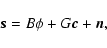$$\vec{s}=B\phi+G\vec{c}+ \vec{n},$$ (9)

where s is the m-element column vector of WFS measurements, c the n-element vector of DM actuator commands, G the $m\times n$ DM interaction matrix (m rows, n columns), B the $m\times N$ phase interaction matrix and n a m-element vector of additive noise on the measurement signal. G and B are Jacobian type matrices, $G=\partial\vec{s}/\partial\vec{c}$ and $B=\partial\vec{s}/\partial \phi$, encoding information on the geometry of WFS sub-apertures and DM influence functions. Whereas B is of primarily academic interest, G is a calibration matrix that defines the fundamental interaction between the deformable mirror and the wavefront sensor. It may be obtained column-wise by poking the DM actuators one by one and measure the response in the sensor (hence called the "poke-matrix'' by some authors).

2.2 Wave-front reconstruction

To spatially control an adaptive optics system, the inverse problem posed by the linearized interaction Eq. (9) must be solved for the command signal vector c. Requiring the reconstruction to be a linear mapping, the solution may be stated on the general form

$$\vec{c}=F\vec{s},$$ (10)

where F is a spatial-temporal filter. Defining the open loop measurement signal $\vec{s}_0=B\phi+ \vec{n}$, one finds upon combining (10) and (9)

$$\vec{c}=(FG-I)^{-1}F\vec{s}_0.$$ (11)

From here it is not clear how to proceed in the general case to derive the filter F that is closed loop optimal. Ellerbroek (1994) shows that an optimal estimator may be derived by separating spatial and temporal variables by the splitting F=fE, where f is a scalar temporal filter and E the spatial reconstruction matrix, and then imposing the constraint EG=I to linearize the spatial component of (11). For reasons of sparseness and computational efficiency (see Sect. 3), only open loop wavefront reconstruction shall be considered here. Open loop estimators may be sought by solving the simplified interaction equation

$$\vec{s}=G\vec{c}+\vec{n}$$ (12)

for the command signal vector c. To date, a commonly used technique is to ignore the noise component and invert the interaction matrix G by singular value decomposition (SVD) and filtering, whereupon wavefront reconstruction may be conducted by the simple matrix-vector multiplication $\vec{c}=E\vec{ s}$. The computational costs associated with this type of wavefront reconstruction are listed for an assortment of AO and MCAO configurations in Table 1. The SVD estimator is a least-squares solution which minimizes the merit function $\vert\!\vert\vec{s}-G\vec{c}\vert\!\vert^2$. There are several reasons to look beyond the SVD estimator, however, and consider adding a few layers of sophistication:

1.

For very high-order systems it might be necessary to filter many modes which, even though poorly sensed, may constitute a non-negligible fraction of the modal content of the turbulence-induced aberrations. Indiscriminate filtering of singular modes will gradually reduce the modal efficiency of the wavefront reconstruction.

2.

The least-squares estimator minimizing $\vert\!\vert\vec{s}-G\vec{c}\vert\!\vert^2$ is a purely geometric reconstructor that does not take into account potentially useful a priori knowledge about statistics of the noise in the WFS or turbulence in the atmosphere, which could help to condition the over-determined system and improve performance and robustness.

3.

As explicit matrix inversion, a full SVD is an O(n³) computation that takes no advantage of sparseness. For extremely high-order systems, a computational problem will arise in real-time control as well as in simulations.

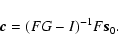
One may solve the inverse problem posed by (12) by a Bayesian approach that delivers a least-squares estimator weighted by noise statistics and regularized by open loop turbulence statistics. This estimator is derived in Appendix A, and the regularized inverse problem is given by the expression (A.10)

$$(G^TC_n^{-1}G+C_c^{-1})\vec{c}=G^TC_n^{-1}\vec{s},$$ (13)

where $C_n=\langle\vec{n}\vec{n}^T\rangle$ is the WFS noise covariance matrix and $C_c=\langle\vec{c}\vec{c}^T\rangle$ is the actuator command signal covariance matrix. By inverting the left-hand matrix one obtains the standard Wiener filter, sometimes referred to as the maximum a posteriori (MAP) estimator (Fusco et al. 1999). Assuming Kolmogorov turbulence statistics, one may estimate C_c^-1 by projecting the turbulence onto a Zernike modal basis, for which the covariances were worked out by Noll (1976). Introducing the pupil-plane phase bases H and Z of DM influence functions and Zernike modes, a turbulence-induced phase aberratio $\phi$ may be described in either base as $\phi=H\vec{c}=Z \vec{a}$, where a is the vector of Zernike coefficients. Forming the inverse composite mapping $\vec{c}=(Z^TH)^{-1}\vec{a}$ it is clear that C_c in general can only be found up to least-squares fit, but its inverse has the exact representation

 

C_c^-1=H^TZC_a^-1Z^TH, (14)

which is accurate up to the numerical orthonormality of the Zernike modes in Z, and $C_a=\langle\vec{a}\vec{a}^T\rangle$. It may be noted for future reference that the DM interaction matrix may be represented by the composite mapping G=AH.

Figure 2: Upper left - Fried geometry of WFS sub-apertures and DM actuators; upper right - the natural numbering of the actuators. Lower left - heuristic model for a Fried geometry interaction; numbers indicate the x- and y-component of the gradient registered in respective sub-aperture as a result of poking the central actuator. Lower right - numerical weights for the discrete definition C of the Laplacian curvature operator, for an internal, edge and corner point of the mesh.

Open with DEXTER

3 Efficient performance estimation

3.1 Sparse wave-front reconstruction

Crucial to the numerical simulation to be presented here is the use of sparse matrix methods for wavefront reconstruction, which in turn relies on the matrices involved actually being sparse. So far nothing has been said about the morphology of the interaction matrix G or the covariance matrices C_n and C_c, and what about them might potentially invite the use of sparse techniques. The particular form of these matrices depends strongly upon the type of wavefront sensor and deformable mirror being used, and their relative geometry as embodied in the interaction matrix. For the high-order AO applications we wish to investigate, it is reasonable to make the following assumptions:

• The influence functions $g_j(\vec{x})$ are localized, extending no further than the immediate nearest neighbor.
• A Fried or Hudgin geometry of actuators and sub-apertures in perfect alignment (no DM-to-WFS misregistration).
• Identical influence functions, $g_j(\vec{x})=g(\vec{x})*\delta(\vec{x}-\vec{x}_j)$, with perfect x and y symmetry.

The first assertion comes from the difficulty of building bimorph or electrostatic membrane DMs of very high order. This makes it plausible that piezostack, electrostatic PMN (lead-magnesium-niobate) or MOEM (micro-opto-electro-mechanical) type DMs will be employed for high-order systems, whose actuators have a well localized influence and produce thus a sparse WFS response. For manufacturing reasons, it is also reasonable to assume a square geometry of DM actuator and WFS sub-aperture patterns such as e.g. the Fried configuration drawn in the upper part of Fig. 2 - hexagonal patterns are a possible alternative with some attractive features, but they would not affect the sparse wavefront reconstruction to be presented here dramatically, only complicate the numerical analysis considerably. In both the Fried and Hudgin configurations the inter-actuator and sub-aperture spacings are matched, with the actuators positioned either at the corners of the sub-apertures (Fried) or along the sides (Hudgin) bisecting the sub-aperture. As a final assumption, a Shack-Hartmann type wavefront sensor shall be adopted, which measures a two-component gradient in each sub-aperture. It is clear from these assumptions that the interaction matrix G will have no more than eight nonzero entries per column (i.e. per actuator), making it and its covariance G^TG very sparse. The drawing on the lower left of Fig. 2 illustrates the idealized heuristic interaction model that was adopted based on these assumptions: any given actuator on the DM will produce x- and y-gradients of equal amplitude but alternating sign in the sub-apertures that lie within the actuator's region of influence.

To quantify the sparseness of a matrix one may define the degree of sparseness $\chi$ as the number of zeros divided by the total number of elements - the sparser a matrix, e.g. the closer to one $\chi$ becomes, the greater the gain of sparse methods over explicit ones. Assuming the noise in different sub-apertures of the WFS to be uncorrelated, C_n will be diagonal with the individual sub-aperture variances  $\sigma_i^2$ on the diagonal, making C_n a maximally sparse full-rank matrix. If in addition the sub-aperture noise variances are all the same $\sigma_i^2=\sigma_n^2$ (as follows upon assuming identical detector pixels and ignoring the effects of partial illumination at the edge of the aperture), then $C_n^{-1}=\sigma_n^{-2}I$, where I is the identity matrix. The regularization term $C_{\phi}^{-1}=\langle\phi\phi^T\rangle$, however, is a full matrix and some approximation must be employed to render it sparse. It was demonstrated by Ellerbroek (1986,2002) that approximating the Kolmogorov turbulence power spectrum by $\Phi(\kappa)\propto\kappa^{-11/3}\approx\kappa^{-4}$, where $\kappa$ is the radial component of the spatial frequency, yields a sufficiently sparse approximation to  $C_{\phi}^{-1}$ of the form

$$C^{-1}_{\phi}\approx \alpha C^TC,$$ (15)

where C is the discrete matrix representation of the Laplace curvature operator $\nabla^2$ and $\alpha$ a scalar parameter. By Taylor expansion, a second-order accurate finite-difference approximation to the two-dimensional Laplacian is given by

$$\left.\nabla^2\! \phi (x,y)\right\vert _{k,l}=\left.\left(\frac{\... ... _{k,l} \propto\phi_{k+1,l}+\phi_{k-1,l}-4\phi_{k,l}+\phi_{k,l+1}+\phi_{k,l-1},$$ (16)

where the paired indices (k,l) refer to the discrete x- and y-coordinates (x_k,y_l) in the pupil plane. Hence, C will have no more than five nonzero elements per column, which makes it and C^TC very sparse matrices as soon as the order of the system reaches nontrivial proportions. It was also verified by Ellerbroek (2002) that simple boundary conditions such as mirroring or protruding from the center produce sufficiently good results that one need not look into more sophisticated extrapolations at the edge of the pupil (the drawing on the lower right of Fig. 2 illustrates the boundary conditions applied here for edge- and corner points). This and the fact that the turbulence approximation  $11/3\approx4$ works admirably are not so surprising, since the role of the regularization term C_c^-1 was never to perfectly tell the system exactly how to reconstruct turbulence from WFS signals. Its main job is merely to support the inversion by smoothing out singularities and, in the presence of noise, to provide some additional advice on what to do, in a statistical sense, with noisy measurements. Multiplying out the noise variance  $\sigma_m^2$, the approximate wavefront reconstruction equation with all sparse matrices is thus finally obtained as

$$(\underbrace{G^TG+\alpha C^TC}_{A})\vec{c}=G^T\vec{s}.$$ (17)

where $\alpha\propto\sigma_m^2r_0^{5/3}$, and r₀ is the Fried parameter governing the turbulence strength. The resultant system matrix $A=G^TG+\alpha C^TC$ is shown in Fig. 3 for two systems with eight (n=69) and 32 (n=877) sub-apertures across the telescope aperture. For the n=877 actuator system A attains a sparseness of $\chi=98.6$%, which already suggests the use of a sparse algorithm to economize on computations, even though conventional reconstruction would not be a computational problem at this level. A useful feature of implicit wavefront reconstruction schemes is that small adjustments may be made to the constituent matrices in order to optimize the reconstruction in real-time. Equation (17) provides a clear example: as was mentioned in the introduction, the influence of the regularization term is controlled by a single parameter $\alpha$, which may be adjusted on the fly to match the current atmospheric seeing and WFS noise conditions - in explicit wavefront reconstruction one would have to recompute the reconstructor E by SVD or matrix inversion each time an adjustment was made (with a Cholesky solver one would need to compute the factorization again).

	Figure 3: Modulus of GTG+CTC for n=69 and n=877.
Open with DEXTER

Figure 4: Required computing time $\log t$ as a function of the order $\log n$ of the system for explicit (pluses) matrix-vector multiplication and sparse (diamonds) PCG wavefront reconstruction algorithms. Slopes extrapolated from the last two data points are indicated next to each data set, where the two values for the PCG, 1.56 and 1.18, correspond to relative error tolerances of 10-6 and 10-2.

Open with DEXTER

Conjugate gradient (CG) methods provide a quite general means to solve linear systems of the form (17) by iteration. Given an initial guess for the solution vector c, the CG algorithm generates a succession of orthogonal search directions that produce gradually improved estimates $\vec{c}_*$, and the recurrence may be terminated when sufficient accuracy is achieved. For the numerical simulation of this study, the preconditioned conjugate gradient (PCG) method described in Press et al. (1992) was employed. The PCG algorithm deviates from the CG only by both sides of (17) being pre-multiplied by the inverse of a "preconditioning matrix'' $\widetilde{A}$, which was taken to be simply the diagonal part of the system matrix A. The PCG algorithm turns out to be particularly suitable for sparse systems, as the matrix A is only referred to by its multiplication with a vector, which can be very efficiently implemented for a properly stored sparse matrix. The sparse storage scheme adopted for this study, the row-wise format described in e.g. Pissanetzky (1984), is in fact constructed such that the efficiency of the matrix-vector multiplication is optimized with respect to sparseness. A representative benchmarking of the sparse PCG applied to the current task of AO wavefront reconstruction is shown in Fig. 4. Error tolerances of 10^-6 and 10^-2 were bench-marked, where the latter leads to the PCG computational cost scaling almost linearly (exponent 1.18) with n. As is shown in Sect. 4, other error sources present in the adaptive optics system relax the requirements on precision in the reconstruction algorithm, such that a remarkably large intrinsic error (e.g. $\sim$10^-2) may be tolerated without significant loss of AO performance.

3.2 Monte Carlo simulation

The numerical Monte Carlo simulation is of the type described in, e.g., Flicker et al. (2000), as originally devised by Rigaut (1999) for MCAO feasibility studies at the Gemini Observatory. The designation "Monte Carlo'' is here used in its loosest sense, that the statistically averaged result is obtained after processing a large number of random inputs. Its main components are sketched in Fig. 5, which reflects the system architecture as depicted in Fig. 1. The main differences in the current study from previous applications of the algorithm lies within the propagation module, the WFS module and the wavefront reconstruction algorithm that was described in the previous Section. The atmosphere is modeled by a finite number of infinitesimally thin layers of turbulence producing pure phase aberrations $\phi$, that are stacked vertically at varying altitudes above the telescope. The phase aberrations obey von Kármán statistics $\Phi_{\phi}(\kappa)\propto(\kappa^2+\kappa_0^2)^{-11/6}$, with an outer scale $L_0=\kappa_0^{-1}$ ranging between 25-100 m in the various simulations presented in Sect. 4. The propagation operator ${\cal K}$ would in the general case be a Fresnel propagator that propagates a plane wave over the atmospheric aberrations $\phi$ and the adaptive phase corrections $\varphi$ into a residual complex aberrated wave  $\varepsilon$ in the telescope pupil plane. Under assumptions of weak and not extremely high-altitude turbulence, however, one may forego a wave optical description and model propagation geometrically as the linear addition of phase perturbations. This neglects the effects of scintillation, which are small at near-infrared wavelengths, 1-2.2 $\mu$m, but become important at visible wavelengths and when high a degree of correction is the goal (Flicker 2001; Sasiela 1994).

	Figure 5: Flow diagram of the hybrid numerical simulation.
Open with DEXTER

The WFS module is of a fundamentally different function in this simulation than previous ones. Rather than building a wave optical model for a sub-aperture of the Shack-Hartmann sensor, the WFS signal s is here obtained from the residual phase $\varepsilon$ directly by a sparse matrix-vector multiplication, ${\bf s}=G_0\mbox{\boldmath {$\varepsilon$ }}$. This is made possible by undersampling the turbulence-induced phase aberrations in the pupil plane - undersampling in this context meaning neglecting spatial frequencies above the cut-off frequency of the DM, which is set by the inter-actuator distance d. This allows the representation in the telescope pupil plane of a DM actuator and a WFS sub-aperture by one single phase-element (pixel). Hence the mapping $H:\vec{c}\mapsto\varphi$ from DM commands to wave-fronts becomes the identity, whereupon G=AH=A, according to the discussion directly following Eq. (14). Equating phase and actuator commands, it follows from the interaction Eq. (12) that both are mapped into WFS signals by the interaction matrix G. Hence the WFS model $\vec{s}=G_0\mbox{\boldmath {$\varepsilon$ }}$, where the subscript zero denotes the pupil-plane interaction, in order to distinguish it from conjugate-plane interactions that enter into G when looking to MCAO configurations. Undersampling this coarsely is a rather crude approximation that will not produce very accurate results unless compensated for. Two obvious errors thus unaccounted for are the fitting of DM influence functions to phase aberrations and the spatial aliasing of high spatial frequencies in the WFS. Presently, only simple analytical models are applied to account for the fitting error phase variance $\sigma^2_{\perp}$ in the limit of long exposure time, and the contribution to the WFS measurement signal from spatial aliasing (see next section). The remainder of the simulation sequence sketched in Fig. 5 is straightforward. Noise and aliasing vectors n and r are added to the obtained WFS signal

$$\vec{s}=G_0\mbox{\boldmath {$\varepsilon$ }}+\vec{n}+\vec{r},$$ (18)

and the sum is pre-multiplied by G^T to prepare the vector b that is input into the sparse PCG wavefront reconstruction algorithm. The PCG delivers the required actuator adjustment c, which is added to the current shape of the DM by a standard integrating controller over a scalar gain g. The operator ${\cal T}$ shifts the turbulence screens according to wind velocity vectors before evaluating performance in terms of the field-dependent pupil-plane residual phase variance  $\sigma _{\varepsilon }^2$. It merits comment that, in this hybrid model, aliasing enters the interaction on exactly the same basis as noise, although with different spatial statistics.

3.3 Fitting and aliasing compensation

It remains to be investigated how first-order system errors such as servo-lag and anisoplanatism are affected by the truncation of high spatial frequencies, but it is verified in Sect. 4 that these effects are minor. The DM fitting error will here be approximated as the total phase variance deriving from spatial frequencies higher than the cut-off frequency  $\kappa_{\rm c}$ of the DM, $\kappa_{\rm c}=(2d)^{-1}$. Integrating the Kolmogorov power spectrum given by Noll (1976) outside the controlled frequency domain gives

$$\sigma^2_{\perp}=\frac{0.023}{r_0^{5/3}}\!\int_{\cal A}\!{\rm d}\mbox{\boldmath {$\kappa$ }}~\kappa^{-11/3},$$ (19)

where $\kappa=\vert\mbox{\boldmath {$\kappa$ }}\vert$ is the radial component of the spatial frequency vector $\mbox{\boldmath {$\kappa$ }}$ and the region ${\cal A}$ is the complement of the centered square with side  $(d\sqrt{2})^{-1}$. Evaluating the integral in cylindrical coordinates  $(\kappa,\theta)$ and observing the radial symmetry gives

 

$$\sigma^2_{\perp} 8\times\frac{0.023}{r_0^{5/3}}\!\int_0^{\pi/4}\!\!\!{\rm d}\theta\!\int_{\kappa(\theta)}^{\infty}\!\!{\rm d}\kappa~\kappa^{-8/3}$$ = (20)

$$\frac{24}{5}\times\frac{0.023}{r_0^{5/3}}\times({d}\sqrt{8})^{5/3}\!\int_0^{\pi/4}\!\!{\rm d}\theta~\cos^{5/3}\!\theta$$ = (21)

$$\approx 0.414\left(\frac{d}{r_0}\right)^{5/3},$$ (22)

where the azimuthal integral was numerically integrated to 0.663, and the cosine derives from the boundary  $\kappa(\theta)$ of ${\cal A}$ in the interval $\theta\in[0,\pi/4]$ described in polar coordinates as $\kappa(\theta)=(d\sqrt{8}\cos\theta)^{-1}$. This 5/3' s power law $\sigma^2_{\perp}=a(d/r_0)^{5/3}$ may be applied with various coefficients a that better approximate the real fitting of different types of influence functions. Coefficients for the most common types are listed in e.g. Hardy (1998), but in this paper the value 0.414 as derived in (22) will be used throughout. This result applies less well in the case of multi-conjugation, but it shall be used nevertheless as a rough approximation - the method in Rigaut et al. (2000) could plausibly lead to a better estimation in this case.

The WFS spatial aliasing error is produced by some of the high spatial frequency content of the atmospheric turbulence being folded into the interval $[-\kappa_{\rm c},+\kappa_{\rm c}]$ by the discrete sampling of the wavefront. Since those high frequencies that produce aliasing remain largely unattenuated by the AO system, open loop statistics may be employed to represent aliasing to first order. Approximating the Shack-Hartmann WFS by an infinite array of gradient sub-apertures of linear dimension d, the aliasing measurement signal  $\vec{m}_{\perp}$ as a function of the pupil plane coordinate x may be expressed as

$$\vec{m}_{\perp}(\vec{x})=~~\mathrel{ \raise0.pt\hbox{\rlap{\h... ...ght)*\mbox{\boldmath {$\nabla$ }}\phi_{\perp}(\vec{x})\right],$$ (23)

where asterisk (*) denotes convolution, $\Pi$ is the square windowing function defining one sub-aperture, $\phi_{\perp}$ is the high-frequency component of the phase and the replicating function (the shah) was defined as

$$\mathrel{ \raise0.pt\hbox{\rlap{\hbox{\hbox{$\coprod$ }}}\hsk... ...{n=-\infty}^{+\infty}\delta\left(\frac xd-m,\frac yd-n\right).$$ (24)

As the shah is its own Fourier transform (Bracewell 1994), the spatial Fourier transform of the measurement becomes

$$\widetilde{\vec{m}}_{\perp}(\mbox{\boldmath {$\kappa$ }}) \mathrel{ \raise0.pt\hbox{\rlap{\hbox{\hbox{$\coprod$ }}}\hskip5.... ...dmath {$\kappa$ }}\widetilde{\phi}_{\perp}(\mbox{\boldmath {$\kappa$ }})\right]$$ = (25)

$$\sum_{m=-\infty}^{+\infty}\sum_{n=-\infty}^{+\infty}\!\!{\rm i}\vec{k}~ {\rm sinc}(k_m)~{\rm sinc}(k_n)~\widetilde{\phi}_{\perp}(\vec{k}),$$ = (26)

where the aliased frequency vector k was defined as

$$\vec{k}=(k_m,k_n)=\left(\kappa_x-\frac md,\kappa_y-\frac nd\right),$$ (27)

and ${\rm sinc~(\vec{x})=\sin~(\pi \vec{x})/~(\pi \vec{x})}$. The phase spectrum may be written $\widetilde{\phi}_{\perp}=\vert\widetilde{\phi}_{\perp}\vert\exp({\rm i}\psi)$ where $\psi$ is the phase shift of the complex spectrum $\widetilde{\phi}_{\perp}$. Whereas the modulus $\vert\widetilde{\phi}_{\perp}\vert$ inherits the Gaussian statistics of $\phi$, $\psi\in[0,2\pi]$ is uniformly distributed and independent of $\vert\widetilde{\phi}_{\perp}\vert$. Hence the expectation value of $\widetilde{\phi}_{\perp}$ may be split into the separate expectations $\langle\vert\widetilde{\phi}_{\perp}\vert\rangle\langle\exp({\rm i}\psi)\rangle$, where the statistics of $\psi$ lead to the condition

$$\left\langle\exp\left[{\rm i}(\psi_{mn}-\psi_{m'n'})\right]\right\rangle=\delta_{mm'}\delta_{nn'}.$$ (28)

Substituting the von Kármán spectrum from (Noll 1976; Winker 1991) for $\Phi_{\phi_{\perp}}$, the power spectral density (PSD) $\Phi_{\vec{m}}=\langle\vert\widetilde{\vec{m}}_{\perp}\vert^2\rangle$ of $\vec{m}_{\perp}$ evaluates to

 

$$\Phi_{\vec{m}_{\perp}}\!\!\left(\mbox{\boldmath {$\kappa$ }}\righ... ...nc}^2~(k_m)~{\rm sinc}^2~(k_n) 0.023r_0^{-5/3}(k_m^2+k_n^2+\kappa_0^2)^{-11/6},$$ (29)

where $\vert\kappa_x\vert,\vert\kappa_y\vert\le \sqrt{2}\kappa_{\rm c}$. Rather than applying an analytical reconstructor as in (Rigaut et al. 1998) for computing the aliasing phase variance, the PSD (29) will here be used to generate the aliasing vector r indicated in (18) by Fourier transform of $\beta\sqrt{\Phi_{{\vec{m}_{\perp}}}}$, where $\beta$ is a complex-valued white noise. By doing so, the WFS aliasing is propagated through the PCG wavefront reconstructor to produce a resultant effect on the DM commands that observe the proper propagation properties.

Figure 6: Residual phase variance $\sigma ^2_{\varepsilon }$ and number of PCG iterations versus the PCG relative error tolerance, for the $12\!\times\!12$ Shack-Hartmann test configuration in conventional AO (dotted lines) and MCAO (dashed lines) mode. In the top field, a field-weighted average (pluses), an unweighted average (diamonds) and the on-axis value (asterisks) are plotted for comparison.

Open with DEXTER

Table 2: Discrete 4-layer model for atmospheric turbulence - h is the layer altitude, $C_n^2/\mu _0=f$ is the fractional turbulence strength per layer, and v is the wind speed.

  
4 Model implementation

Simulation results for a number of different AO and MCAO configurations are presented at the end of this section. Of particular interest are the results concerning extremely high-order systems, and the investigations into scaling laws for AO performance with telescope diameter D and with turbulence outer scale L₀. The simulations all employ a generic four-layer atmospheric model, with parameters as summarized in Table 2. The altitude h refers to the level above the telescope site, and the fractional turbulence strength f_l per layer l is defined as $f_l=c_l/\sum_l c_l$, where the c_l are the coefficients of the C_n² decomposition $C_n^2(h)=\sum_l c_l\delta(h-h_l)$. In terms of the $0{\rm th}$ turbulence moment $\mu_0=\int\!{\rm d}h~C_n^2(h)$, these coefficients are given by $c_l=\mu_0f_l$. The wind speeds v_l were given random directional vectors from a uniform distribution. It should be noted that, although this toy atmospheric model does not derive from real measurements, it was contrived to be conservative with respect to reported atmospheric conditions at most good astronomical observing sites, without for that reason being overly pessimistic. Where nothing else is stated, other observation and simulation parameters assumed the values listed in Table 3. Only a 2-DM case was considered for the MCAO simulations, and the guide star magnitudes were all set to 10 in order to suppress the effects of photon noise (CCD read-out noise was not included in the simulation) - the main effects investigated for this study were the errors associated with LGS (cone effect), MCAO (tomographic error) and the outer scale of turbulence L₀.

Table 3: Observational and system simulation parameters.

4.1 Efficiency optimization

In order to optimize the efficiency of the PCG wavefront reconstruction algorithm, its required accuracy in an AO simulation was metered versus its relative error tolerance. Since the error tolerance determines when to terminate the recursion, it directly governs the computational cost for wavefront reconstruction. The somewhat surprising results are shown in Fig. 6, where the upper part plots the residual pupil plane phase variance $\sigma ^2_{\varepsilon }$ versus PCG error tolerance, and the lower part plots the average number of required PCG iterations. Both a conventional AO (dotted lines) and a MCAO (dashed lines) system of the same order (the $12\!\times\!12$ Shack-Hartmann used for the comparison in Fig. 7) were tested for comparison. It is seen that over a range of 10⁷ increase in the error tolerance, over which the PCG iteration count drops by roughly a factor of 100, there is very little loss of AO performance - superimposed upon a very mild and gradual increase in $\sigma _{\varepsilon }^2$ there is an irregular jitter of comparable or even larger magnitude. With turbulence variations sufficiently averaged (100 independent atmospheric realizations with 2000 Monte Carlo cycles averaged within each), this jitter can only be numerical, pertaining to the inner machinations of the PCG. The investigation of AO performance versus PCG error tolerance was discontinued at a value of 0.2, as at this level the computational cost of the PCG reconstruction in the case of the conventional AO system was already down to a single PCG iteration upon the initial guess. The simulation results presented in this section were produced at a PCG relative error tolerance of 0.01, where the scaling with n for large systems is approximately  O(n^1.2) as shown in Fig. 4.

	Figure 7: Comparison between simulation results (phase variance - solid; Strehl ratio - dotted) for the hybrid simulation of the current study (diamonds) and a more accurate wave optical simulation with well-sampled turbulence (pluses). Dashed curves show for comparison the hybrid simulation result without fitting and aliasing compensation.
Open with DEXTER

4.2 Model validation

The efficient simulation model was corroborated for realism and accuracy versus a full-fledged wave optical Monte Carlo simulation of similar type, where all the first-order errors (fitting, aliasing, servo-lag, anisoplanatism and noise) are modeled with high accuracy. For the comparison, a small test configuration ( $12\!\times\!12$ Shack-Hartmann WFS, n=137) on an 8-m telescope was simulated, and the comparison is shown in Fig. 7. Looking to the curves of residual phase variance $\sigma _{\varepsilon }^2$ (solid lines) versus angle from the guide star, it is observed that the efficient simulation is afflicted with a bias of approximately 0.04 rad². The majority of this offset is due to the analytical fitting and aliasing compensation, which in their approximation do not exactly reproduce the conditions in the more accurate simulation. There is an additional variation across the field, and at the edge of the field the discrepancy is close to 0.1 rad², but looking to the Strehl curves (dotted lines) this discrepancy translates to less than 5% relative deviation over the range of values plotted (35 arcsec), with a field average of 3%. These numbers are quite tolerable for a first-order performance estimation model, and it may be concluded that undersampling the frequency content of the atmospheric turbulence to first order has no or only a negligible impact on the errors associated with anisoplanatism, servo-lag and noise. While small in the present context, these discrepancies may not be completely insignificant for a tight error budget as far as the design of a real system is concerned. For that purpose one would need to look into second-order corrections to improve upon the accuracy of the model, if the current hybrid algorithm is to be used. Presently, no higher-order correction schemes have been investigated. Keeping in mind that fitting and aliasing are given by analytical approximations and that scintillation remains unaccounted for, simulation results for a number of relevant AO and MCAO configurations are presented in the following.

   
4.3 Laser beacons and multi-conjugation

Concerning laser guide stars and multi-conjugated systems, a few special considerations must be taken in order to ensure that these are efficiently implemented without losing accuracy in the simulation.

1.

For the case of laser guide star (LGS) adaptive optics, the propagator ${\cal K}$ must include a scaling procedure in order to account for the cone effect that arises when using a reference beacon at a finite altitude. The horizontal scaling of the atmospheric turbulence is accomplished by rebinning the phase screens (which are periodic) onto a finer mesh and resample at new coordinates by cubic spline interpolation. Tip and tilt modes were filtered from the measurement signal s rather than being projected out of the controlled subspace of the interaction matrix G, which would render it non-sparse, and a NGS employed for tip-tilt sensing.

2.

For the case of multi-conjugated adaptive optics (MCAO), the interpolation described above would be subject to aliasing effects at the edges of the DMs if applied thereto, and should be avoided if possible. Accuracy in the wavefront sensing is thus retained by having the guide star positions on the sky observe integer pixel shifts on the conjugated DMs. The integrated DM correction in the direction of any guide star may then be obtained by adding the DM shapes conformally without interpolation.

3.

For the case of LGS MCAO, the pixel scales at the conjugated DMs were reduced by the geometric factor 1-h_k/H, for a LGS at the range H and a DM at the range h_k. By having the LGS positions on the sky correspond to integer pixel shifts on the conjugated DMs with this reduced scale, the DM phase may be summed as in the NGS MCAO case and only the turbulence interpolated. Differential tilt is in this case obtained from three tip-tilt NGS, and compensated using a separate control loop (Ellerbroek & Rigaut 2001).

	Figure 8: On-axis residual phase variance $\sigma _{\varepsilon }^2$ versus telescope diameter D for LGS AO, for a range of outer scales L0. Low- and high-order AO systems with d=0.8 m (solid) and d=0.5 m (dashed) are both shown for comparison.
Open with DEXTER

4.4 Sample numerical results

As the diameter of the telescope aperture D approaches the turbulence outer scale L₀, low-order modes responsible for a large fraction of the turbulent energy such as tip and tilt, defocus, astigmatism etc. become de-weighted relative to higher order modes within the aperture. Although L₀ is a poorly known quantity at most sites and times, its value seems to be of critical importance to the design and performance of ELTs. Predictions based in Kolmogorov theory do no longer apply, but it has not been investigated extensively how the characters of angular and focal anisoplanatism scale to ELTs, especially when it comes to tomography and MCAO. Figures 8 and 9 plot the residual phase variance  $\sigma _{\varepsilon }^2$ for two conventional LGS AO systems with d=0.8 m and d=0.5 m as the telescope diameter was varied through D=[10,30,50,100] m. Since performance is measured only on the axis of the LGS, angular anisoplanatism is not present, and for the relatively benign observation scenario chosen (near-infrared, bright guide stars - see Table 2) the noise error is negligible and the servo-lag error small. The dominant error sources in Figs. 8 and 9 are therefore DM fitting and LGS focal anisoplanatism, and for small D ($\le$10 m) the cone effect is mild enough compared to the fitting error that no variation with L₀ is observed. According to Kolmogorov theory, the fitting error does not vary with telescope diameter when aperture filtering is not taken into account (and only weakly when it is), and the induced phase variance due to the cone effect should scale as D^5/3 (Fried & Belsher 1994). The increase in $\sigma ^2_{\varepsilon }$ in Fig. 8 therefore chiefly reflects the cone effect, but in part also the much smaller variations of the servo-lag, aliasing and reconstruction errors that arise with the departure from Kolmogorov statistics when the telescope diameter approaches the outer scale. As seen from the log-log presentation, however, the residual phase variance for the various cases still scales very much like a power law with a varying exponent. By assuming a power law relation of the form $\sigma _{\varepsilon }^2\propto D^{\gamma }$ and fitting straight lines to the logarithmized data in Fig. 9, one may obtain the exponent $\gamma$. The exponents for the current data are listed in Table 4, and the deviations from the 5/3's law predicted by Kolmogorov theory are seen to be significant.

	Figure 9: Same data as in Fig. 8 re-plotted on logarithmic axes to show the differing slopes.
Open with DEXTER

Table 4: Estimated exponents $\gamma$ in a power-law fit of $\sigma _{\varepsilon }^2\propto D^{\gamma }$.

This is partially due to the finite outer scale, but as may be inferred from the two columns of the table, also dependent upon the inter-actuator density d. Not simply does the AO residual phase variance depend upon the outer scale, but more precisely it depends upon the resultant spatial statistics as the turbulence is projected onto the influence functions of the DM (or equivalently, the controlled modes of the wavefront estimator). The smaller the inter-actuator distance d, the higher the spatial cut-off frequency of the deformable mirror and the closer to the real turbulence spectrum the system operates. That $\gamma$ decreases when d increases can be understood in terms of the AO system addressing less of the high spatial frequency content of the atmosphere as the order of the system goes down. With a finite outer scale, the deviations from Kolmogorov statistics then become increasingly more prominent among the low spatial frequencies that are compensated by the system. It may be inferred by numerical evaluation of turbulence integrals (Sasiela 1994)

Table 5: Strehl ratio simulation results for 2-DM MCAO system with 5 NGSs or 5 LGSs and three different turbulence outer scales L₀. For the case d=0.5 m (left-hand side of table), the square field of view defined by the guide stars measured 40 arcsec in the NGS case and 36 arcsec in the LGS case. For the d=0.8 m case, the field was 67 and 60 arcsec for the NGS and LGS simulations.

that include a finite outer scale, that the contribution to $\sigma _{\varepsilon }^2$ due to focal anisoplanatism will be reduced at large D and small L₀ as compared to Kolmogorov theory. Where this effect becomes significant, the scaling with D will start to deviate from a simple power law. There is an indication to this effect by the presence of an inflection point in some of the curves. The current sparse data does not allow a detailed analysis of this phenomenon, however, and a discussion of thereof is in any case beyond the scope of the present study.

A series of MCAO cases with two DMs, conjugated to zero and 10 km, and either five NGSs or five LGSs in a X-like geometry with a base of 40'' were simulated subject to the same variations in L₀ and d as the single LGS simulation. The tomography algorithm employed was the linear MAP estimator described in Sect. 2.2, which is derived in Appendix A. The results are given in Table 5, in the form of the field-averaged Strehl ratio $\bar{S}$ (left column) and the relative deviation over the field $\delta S/\bar{S}$ (right column). The Strehl ratios were computed from the phase variance in the extended Maréchal approximation, $SR\approx\exp(-\sigma_{\varepsilon}^2)$, which means that entries below 0.2 are somewhat underestimated. For MCAO, no analytical predictions for the tomographic error in Kolmogorov theory have been produced, leaving little by which to compare these results. It may be conjectured, however, that the instance of tomography should help to mitigate the cone effect even further upon the aid lent by the finite outer scale. Comparing with the values in Fig. 8, it is seen that the sensitivity to L₀ is stronger in the MCAO case, plausibly due to the larger field over which MCAO attempts to compensate turbulence. The gain toward low L₀ is however also larger for LGS MCAO than LGS AO, indicating a very nonlinear coupling between L₀, D and the instance of tomography and multi-conjugation - which is why results for ELTs are very difficult to infer with any confidence from simulations at smaller scales. It is seen that, contrary to some claims in the literature based on very conservative estimations or extrapolations, a small number of LGSs may actually provide a useful level of compensation on telescopes as large as 30-50 m, if not close to diffraction-limited. For higher LGS performance the LGS density must be increased in order to reduce the tomographic error due to focal anisoplanatism, which means a larger number of LGSs if a given field of view is to be maintained. Tilt anisoplanatism in LGS-based MCAO systems will reduce performance somewhat with respect to NGS MCAO, as discussed in Ellerbroek & Rigaut (2001). Regarding concerns occasionally voiced that LGS tomography, tilt anisoplanatism aside, would be implicitly less accurate than NGS tomography, no such effect has been ever observed by the author of this paper. It has been verified in a designed test simulation that, if the turbulence was confined to the union volume spanned by the cones (i.e. no unsampled turbulence), LGS and NGS tomography become exactly equivalent. The poorer performance of LGS tomography in a real scenario is solely due to the loss of information that a focused sensor beam must contend with, and minimizing this information loss by increasing the LGS density will gradually improve LGS MCAO performance. It remains to be proven however, that an ELT in the range 30-100 m will be able to deliver near-diffraction-limited performance under wind buffeting and mechanical flexure, which may be a larger obstacle to overcome than adaptive optics performance.

5 Conclusions

First-order performance estimation for adaptive optics systems may be accomplished efficiently with a hybrid numerical simulation that combines the accuracy and realism provided by a Monte-Carlo-type simulation with analytical compensation tools where the former was compromised in order to increase efficiency. Systems with $\sim$10⁵ degrees of freedom, including multi-conjugate and laser-guide-star-based systems, may be efficiently investigated thus using a current standard personal computer. Results were presented for a number of AO and MCAO configurations, demonstrating that the turbulence outer scale L₀ has a significant impact on performance when the telescope diameter D approaches L₀. LGS MCAO systems are seen to be more sensitive to L₀ than conventional LGS AO systems, and the gain also larger in MCAO as L₀ becomes smaller. To the best of the author's knowledge, the results for the n=65 282 case represent the largest MCAO system simulated in full to date, although the simulation approaches presented in Ellerbroek (2002) and Gilles et al. (2002) are of comparable capabilities and efficiencies. Future extensions of the simulation will proceed to refine the fitting error estimation and include scintillation effects.

Acknowledgements

The author would like to thank H.-G. Ludwig for many valuable comments on the manuscript and generous support with additional computing resources.

Appendix A: Derivation of maximum a posteriori estimator

The open loop interaction equation may be written

$$\vec{s}=G\vec{c}+\vec{n},$$ (A.1)

from which we wish to estimate the optimal command vector $\vec{c}_*$ that maximizes the a posteriori conditional probability $P(\vec{c}\vert\vec{s})$:

$$\vec{c}_*=\arg\max_{\vec{c}}P(\vec{c}\vert\vec{s}).$$ (A.2)

A standard procedure to find $\vec{c}_*$ that shall be used here is to solve $\partial P(\vec{c}\vert\vec{s})/\partial\vec{c}=0$ for c. From Bayes' theorem of conditional probabilities we have that

$$P(\vec{c}\vert\vec{s})=P(\vec{c})\frac{P(\vec{s}\vert\vec{c})}{P(\vec{s})},$$ (A.3)

where $P(\vec{s})=1$ since this is the measured data and $P(\vec{c})$ is the so-called Bayesian prior, which contains the a priori information on the statistics of $\vec{c}$ that will regularize the solution. Assuming the wave-front sensor sub-aperture noise to be of Gaussian statistics with zero mean and standard deviations $\{\sigma_i\}_{i=0}^{m-1}$, it is seen by rearranging (A.1) that $\vec{s}-G\vec{c}$ shares the statistics of n. Assuming further the noise to be uncorrelated between sub-apertures, $\langle n_i n_j\rangle=\delta_{ij}\sigma_i^2$, the likelihood term $P(\vec{s}\vert\vec{c})$ evaluates to

$$P(\vec{s}\vert\vec{c})=\prod_{i=0}^{m-1}P(s_i\vert\vec{c})$$ (A.4)

$$= \prod_{i=0}^{m-1}\frac{\Delta s}{\sigma_i\sqrt{2\pi}}\exp\!... ...-\frac{1}{2\sigma_i^2}\left[s_i-(G\vec{c})_i\right]^2\right\}$$ (A.5)

$$=\vert C_n\vert^{-1}\left(\frac{\Delta s}{\sqrt{2\pi}}\right)... ...-\frac12(\vec{s}-G \vec{c})^TC_n^{-1}(\vec{s}-G\vec{c})\right],$$

where $C_n=\langle\vec{n}\vec{n}^T\rangle$ is the noise covariance matrix. For mathematical stringency, the term $\Delta s$ specifies the scale of discretization, as the probability would always be zero if the s_i's took on continuous values. Invoking the central limit theorem to bear on refractive index fluctuations in the atmosphere, the open loop statistics of $\vec{c}$ may likewise be assumed to be Gaussian. In analogy with (A.5) we may thus write down the prior term directly as

$$P(\vec{c})\propto\exp\left(-\frac12\vec{c}^TC_c^{-1}\vec{c}\right),$$ (A.6)

where $C_c=\langle\vec{c}\vec{c}^T\rangle$ is the actuator command signal covariance matrix. This gives the a posteriori probability

 

$$% P(\vec{c}\vert\vec{s})\propto\exp\left[-\frac12(\vec{s}-G\vec{c... ...1}(\vec{s}-G \vec{c})\right] \exp\left[-\frac12\vec{c}^TC_c^{-1}\vec{c}\right].$$ (A.7)

Maximizing the probability is equivalent to minimizing the negative of its logarithm, so a local minimum is given where for all vectors u

$$\frac{\partial}{\partial \vec{c}}\ln P(\vec{c}\vert\vec{s})\c... ...c}+\xi\vec{u}\vert\vec{s})-\ln P(\vec{c}\vert\vec{s})}{\xi}=0.$$ (A.8)

It is seen that $\ln P$ is quadratic in c, so taking the derivative will result in a linear equation that should be easy to solve. Evaluating the limit gives

$$\frac{\partial\ln P}{\partial \vec{c}}\cdot\vec{u}=(G^TC_n^{-1}G\vec{c}+C_c^{-1} \vec{c}-G^TC_n^{-1}\vec{s})=0,$$ (A.9)

and a non-trivial solution for all u requires that

$$(G^TC_n^{-1}G+C_c^{-1})\vec{c}=G^TC_n^{-1}\vec{s},$$ (A.10)

from which one may write $\vec{c}_*=E_*\vec{s}$ and identify the MAP reconstructor as E_*=(G^TC_n^-1G+C_c^-1)^-1G^TC_n^-1.

References

 
• Bracewell, R. N. 1994, The Fourier Transform and its Applications, 2nd ed. (WCB/McGraw-Hill Inc.) In the text  
• Cochran, G. M. 1986, Sparse matrix techniques in wavefront reconstruction, Tech. Rep. No. TR-668 (Anaheim, CA-92825, USA: The Optical Sciences Company) In the text  
• Ellerbroek, B. L. 1986, Comparison of least squares and minimum variance wavefront reconstruction for atmospheric turbulence compensation in the presence of noise, Tech. Rep. No. TR-721R (Anaheim CA-92825 USA: The Optical Sciences Company) In the text  
• Ellerbroek, B. L. 1994, J. Opt. Soc. Am. A, 11, 783 In the text NASA ADS  
• Ellerbroek, B. L. 2002, J. Opt. Soc. Am. A, 19, 1803 In the text NASA ADS  
• Ellerbroek, B. L., & Rigaut, F. 2001, J. Opt. Soc. Am. A, 18, 2539 In the text NASA ADS  
• Flicker, R., Rigaut, F., & Ellerbroek, B. 2000, in 4007, Adaptive Optical Systems Technology, Proc. SPIE, 1032 In the text  
• Flicker, R. C. 2001, Opt. Lett., 26, 1743 In the text NASA ADS  
• Fried, D. L., & Belsher, J. F. 1994, J. Opt. Soc. Am. A, 11, 277 In the text NASA ADS  
• Fusco, T., Conan, J., Rousset, G., Mugnier, L. M., & Michau, V. 2001, J. Opt. Soc. Am., 18, 2527 In the text NASA ADS  
• Fusco, T., Conan, J.-M., Michau, V., Mugnier, L. M., & Rousset, G. 1999, Opt. Lett., 24, 1472 In the text NASA ADS  
• Gilles, L., Vogel, C. R., & Ellerbroek, B. L. 2002, J. Opt. Soc. Am. A, 19, 1817 In the text NASA ADS  
• Gilmozzi, R. 2000, in Discoveries and Research Prospects from 8- to 10-Meter-Class Telescopes, ed. J. Bergeron, Proc. SPIE, 4005, 2 In the text  
• Hardy, J. W. 1998, Adaptive optics in astronomy (Oxford University Press), 176 In the text  
• Hawarden, T. G., Dravins, D., Gilmore, G. F., et al. 2002, in Future Giant Telescopes, ed. J. R. P. Angel, & R. Gilmozzi, Proc. SPIE, 4840, in press In the text  
• Le Louarn, M. 2002, MNRAS, 334, 865 In the text NASA ADS  
• Noll, R. J. 1976, J. Opt. Soc. Am., 66, 207 In the text NASA ADS  
• Owner-Petersen, M., & Goncharov, A. 2002, J. Opt. Soc. Am. A, 19, 537 In the text NASA ADS  
• Pissanetzky, S. 1984, Sparse matrix technology (London: Academic Press Inc.) In the text  
• Press, W. H., Teukolsky, S. A., Vetterling, W. T., & Flannery, B. P. 1992, Numerical recipes in C: the art of scientific computing, 2nd ed. (Cambridge University Press) In the text  
• Ragazzoni, R., Farinato, J., & Marchetti, E. 2000, in Adaptive Optical Systems Technology, ed. P. Wizinowich, Proc. SPIE, 4007, 1076 In the text  
• Rigaut, F. 1999, private communication, Gemini Observatory, Hilo-HI, USA In the text  
• Rigaut, F., Salmon, D., Arsenault, R., et al. 1998, Publ. Astr. Soc. Pac., 110, 152 In the text NASA ADS  
• Rigaut, F. J., Ellerbroek, B. L., & Flicker, R. 2000, in Adaptive Optical Systems Technology, ed. P. L. Wizinowich, Proc. SPIE, 4007, 1022 In the text  
• Rigaut, F. J., Veran, J., & Lai, O. 1998, in Adaptive Optical System Technologies, ed. D. Bonaccini, & R. K. Tyson, Proc. SPIE, 3353, 1038 In the text  
• Sasiela, R. J. 1994, Electromagnetic Wave propagation in Turbulence: Evaluation and Application of Mellin Transforms (Springer-Verlag) In the text  
• Snel, R. C., & Ardeberg, A. L. 2002, in Future Research Direction and Visions for Astronomy, ed. A. M. Dressler, Proc. SPIE, 4835, 60 In the text  
• Tokovinin, A., Le Louarn, M., Viard, E., Hubin, N., & Conan, R. 2001, A&A, 378, 710 In the text NASA ADS  
• Winker, D. M. 1991, J. Opt. Soc. Am. A, 8, 1568 In the text NASA ADS