2 The SZ effect for galaxy clusters: A generalized approach

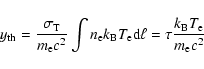
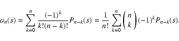
In this section we derive a generalized expression for the SZ effect which is valid in the Thomson limit for a generic electron population in the relativistic limit and includes also the effects of multiple scattering. First we consider an expansion in series for the distorted spectrum I(x) in terms of the optical depth, $\tau$, of the electron population. Then, we consider an exact derivation of the spectral distortion using the Fourier Transform method already outlined in Birkinshaw (1999).

An electron with momentum $p=\beta \gamma$, with $\beta= v/c$ and $\gamma=E_{\rm e}/m_{\rm e}c^2$ increases the frequency $\nu$ of a scattered CMB photon on average by the factor $t \equiv \nu' / \nu = {4 \over 3} \gamma^2 - {1 \over 3}$, where $\nu'$ and $\nu$ are the photon frequencies after and before the scattering, respectively. Thus, in the Compton scattering against relativistic electrons ( $\gamma \gg 1$) a CMB photon is effectively removed from the CMB spectrum and is found at much higher frequencies.

We work here in the Thomson limit, (in the electron's rest frame $\gamma h~\nu \ll ~m_{\rm e}~c^2$), which is valid for the interesting range of frequencies at which SZ observations are feasible.

The redistribution function of the CMB photons scattered once by the IC electrons writes in the relativistic limit as,

$$P_1(s)= \int_0^{\infty} {\rm d}p~ f_{\rm e}(p) P_{\rm s}(s;p),$$ (5)

where $f_{\rm e}(p)$ is the electron momentum distribution and $P_{\rm s}(s;p)$ is the redistribution function for a mono-energetic electron distribution, with $s \equiv \ln(t)$. An analytical expression for the redistribution function of CMB photons which suffer a single scattering, $P_{\rm s}(s;p)$, has been given by Ensslin & Kaiser (2000). The expression for such a redistribution function has been also given analytically by Fargion et al. (1997) and by Sazonov & Sunyaev (2000). Once the function P₁(s) is known, it is possible to evaluate the probability that a frequency change s is produced by a number n of repeated, multiple scattering. This is given by the repeated convolution

 

$$\int_{-\infty}^{+\infty} {\rm d}s_1 \ldots {\rm d}s_{n-1} P_1(s_1) \ldots P_1(s_{n-1}) P_1(s-s_1- \ldots -s_{n-1})$$ P_n(s) =

$$\equiv \underbrace{P_1(s) \otimes \ldots \otimes P_1(s)}_{n{\rm times}}$$ (6)

(see Birkinshaw 1999), where the symbol $\otimes$ indicates each convolution product. As a result, the location of the maximum of the function P_n(s) moves towards higher values of s for higher values of n and the distribution P_n(s) widens a-symmetrically towards high values of s giving thus higher probabilities to have large frequency shifts. The resulting total redistribution function P(s) can be written as the sum of all the functions P_n(s), each one weighted by the probability that a CMB photon can suffer n scatterings, which is assumed to be Poissonian with expected value $\tau$:

 

$$\sum_{n=0}^{+\infty} \frac{{\rm e}^{-\tau} \tau^n}{n!} P_n(s) ={\rm e}^{-\tau} \left[P_0(s)+ \tau P_1(s) + \frac{1}{2} \tau^2 P_2(s)+ \ldots\right]$$ P(s) =

$${\rm e}^{-\tau} \left[\delta(s) + \tau P_1(s) + \frac{1}{2} \tau^2 P_1(s) \otimes P_1(s) + \ldots \right] \cdot$$ = (7)

The spectrum of the Comptonized radiation is then given by

$$I(x) = \int_{- \infty}^{+\infty} {\rm d}s~I_0(x {\rm e}^{-s}) P(s) ,$$ (8)

where

$$I_0(x)=2\frac{(k_{\rm B} T_0)^3}{(hc)^2} \frac{x^3}{{\rm e}^x-1}$$ (9)

is the incident CMB spectrum in terms of the a-dimensional frequency x.

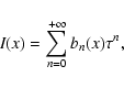
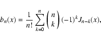
In the following we will derive the expression for the distorted spectrum using first an expansion in series of $\tau$ and then the exact formulas obtained with the Fourier Transform (FT) method.

2.1 High order $\tau$-expansion

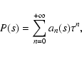
In the calculation of the SZ effect in galaxy clusters it is usual to use the expression of P(s) which is derived in the single scattering approximation and in the diffusion limit, $\tau \ll 1$. In these limits, the distorted spectrum writes, in our formalism, as:

$$I(x) = J_0(x) + \tau \left[ J_1(x) - J_0(x) \right] ,$$ (10)

where

 

$$\int_{-\infty}^{+\infty} I_0(x{\rm e}^{-s}) P_0(s) {\rm d}s = \int_{-\infty}^{+\infty} I_0(x{\rm e}^{-s}) ~\delta(s) ~{\rm d}s$$ J₀(x) =

= I₀(x) , (11)

$$\int_{-\infty}^{+\infty} I_0(x{\rm e}^{-s}) P_1(s) {\rm d}s.$$ J₁(x) = (12)

To evaluate the SZ distorted spectrum I(x) up to higher order in $\tau$, we make use of the general expression of the series expansion of the function P(s)

$$P(s)=\sum_{n=0}^{+\infty} a_n(s) \tau^n ,$$ (13)

which can be written, using Eq. (7), as

$$P(s)=\sum_{k=0}^{+\infty} \frac{(-\tau)^k}{k!} \sum_{k'=0}^{+\infty} \frac{\tau^{k'}}{k'!} P_{k'}(s) .$$ (14)

The general nth order term is obtained by selecting the terms in the double summation which contain the optical depth $\tau$ up to the nth power. These terms are obtained for k'=n-k, and provide the following expression for the series expansion coefficients:

$$a_n(s)=\sum_{k=0}^n \frac{(-1)^k}{k!(n-k)!} P_{n-k}(s) = \fr... ...\begin{array}{c} n \\ k \end{array} \right) (-1)^k P_{n-k}(s).$$ (15)

Inserting the coefficients a_n(s) given in Eq. (15) in Eq. (13) and this last one in Eq. (8), the resulting spectral distortion due to the SZ effect can be written as:

$$I(x)=\sum_{n=0}^{+\infty} b_n(x) \tau^n ,$$ (16)

where the coefficients b_n(x) are given by

$$b_n(x)=\frac{1}{n!} \sum_{k=0}^n \left(\begin{array}{c} n \\ k \end{array} \right) (-1)^k J_{n-k}(x) ,$$ (17)

and

$$J_{n-k}(x)=\int_{-\infty}^{+\infty} I_0(x{\rm e}^{-s}) P_{n-k}(s) {\rm d}s.$$ (18)

In this general approach, we can write the corrections to the distorted spectrum I(x) up to any order n in the quantity $\tau$.

2.2 Exact derivation of the SZ effect

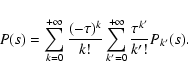
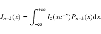
The redistribution function P(s) can also be obtained in an exact form considering all the terms of the series expansion in Eq. (14). In fact, since the Fourier transform (hereafter FT) of a convolution product of two functions is equal to the product of the Fourier transforms of the two functions, the FT of P(s) writes as

 

$$\tilde{P}(k) {\rm e}^{-\tau} \left[1+\tau \tilde{P}_1(k)+\frac{1}{2} \tau^2 \tilde{P}_1^2(k)+\ldots\right]={\rm e}^{-\tau}{\rm e}^{\tau \tilde{P}_1(k)}$$ =

$${\rm e}^{-\tau[1-\tilde{P}_1(k)]} ,$$ = (19)

where

$$\tilde{P}_1(k)=\int_{-\infty}^{+\infty} P_1(s) ~ {\rm e}^{-iks} {\rm d}s~$$ (20)

(Taylor & Wright 1989). The exact form of the Comptonized spectrum I(x) is then given by Eq. (8) in terms of the exact redistribution function

$$P(s) = {1 \over 2 \pi} \int_{-\infty}^{+\infty} \tilde{P}(k)~ {\rm e}^{iks}~ {\rm d}k$$ (21)

which is obtained as the anti Fourier transform of $\tilde{P}(k)$ given in Eq. (19). To compare the exact calculations of the SZ spectral distortion with those obtained in the non-relativistic limit (see Eqs. (1)-(2) as for the thermal case), it is useful to write the distorted spectrum in the form

$$\Delta I(x)=2\frac{(k_{\rm B} T_0)^3}{(hc)^2}y \tilde{g}(x) ,$$ (22)

where $\Delta I(x) \equiv I(x) - I_0(x)$. The spectral shape of the SZ effect is contained in the function

$$\tilde{g}(x)=\bigg( \frac{\Delta I}{I_0}\bigg) \frac{1}{y} \frac{x^3}{{\rm e}^x-1}=\frac{\Delta i(x)}{y}$$ (23)

where $\Delta i\equiv \Delta I \frac{(hc)^2}{2(k_{\rm B} T_0)^3}$. The Comptonization parameter y is defined, in our general approach, in terms of the pressure Pof the considered electron population:

$$y=\frac{\sigma_{\rm T}}{m_{\rm e} c^2}\int P {\rm d}\ell .$$ (24)

2.3 The case of a single thermal electron population

For a thermal electron population in the non-relativistic limit with momentum distribution $f_{\rm e,th} \propto p^2 \exp(-\eta \sqrt{1+p^2})$ with $\eta= m_{\rm e} c^2/k_{\rm B} T_{\rm e}$, one writes the pressure as

$$P_{\rm th}=n_{\rm e} k_{\rm B} T_{\rm e}$$ (25)

and it is easy from Eq. (24) to re-obtain the Compton parameter in Eq. (3) as

$$y_{\rm th}=\frac{\sigma_{\rm T}}{m_{\rm e} c^2}\int n_{\rm e}... ... {\rm d}\ell =\tau \frac{k_{\rm B} T_{\rm e}}{m_{\rm e} c^2}$$ (26)

(we consider here, for simplicity, an isothermal cluster). The relativistically correct expression of the function $\tilde{g}(x)$ for a thermal population of electrons writes, at first order in $\tau$, as:

$$\tilde{g}(x)=\frac{\Delta i}{y_{\rm th}}=\frac{\tau [j_1-j_... ...} c^2}}= \frac{m_{\rm e} c^2}{k_{\rm B} T_{\rm e}}[j_1-j_0] ,$$ (27)

where $j_i \equiv J_i \frac{(hc)^2}{2(k_{\rm B} T_0)^3}$ and the functions J_i are given in Eq. (18).

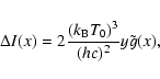
In the same line, it is possible to write the expression of $\tilde{g}(x)$ up to higher orders in $\tau$. For example, limiting the series expansion in Eq. (14) at third order in $\tau$, we found:

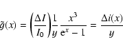
$$\tilde{g}(x)=\frac{m_{\rm e} c^2}{ k_{\rm B} T_{\rm e} } \left[(j... ...frac{1}{2}\tau(j_2-2j_1+j_0) +\frac{1}{6}\tau^2 (j_3-3j_2+3j_1-j_0)\right]\cdot$$ (28)

Notice that while the expression derived for $\tilde{g}(x)$ at first order approximation in $\tau$ is independent of $\tau$, the expression for $\tilde{g}(x)$ at higher order approximation in $\tau$ depends directly on $\tau$. This is even more the case for the exact expression of $\tilde{g}(x)$given in the following. In fact, using the exact form of the function P(s)given in Eq. (22), it is possible to write the exact form of the function  $\tilde{g}(x)$ as:

$$\tilde{g}(x)=\frac{m_{\rm e} c^2}{k_{\rm B} T_{\rm e} } \left... ... i_0(x{\rm e}^{-s}) P(s) {\rm d}s- i_0(x)\right] \right\}\cdot$$ (29)

The expression of $\tilde{g}(x)$ approximated at first order in $\tau$ as given by Eq. (27) is the one to compare directly with the expression of g(x) obtained from the Kompaneets (1957) equation, since both are evaluated under the assumption of single scattering suffered by a CMB photon against the IC electrons. Figure 1 shows how the function $\tilde{g}(x)$ tends to g(x) for lower and lower IC gas temperatures $T_{\rm e}$. This confirms that the distorted spectrum obtained from the Kompaneets equation is the non-relativistic limit of the exact spectrum. Notice that the function $\tilde{g}(x)$ given in Eq. (29) is the spectral shape of the SZ effect obtained in the exact calculation while the function g(x) refers to the 1st order approximated case of a single, thermal, non-relativistic population of electrons.

Figure 1: The function g(x) (solid line) is compared with the function $\tilde{g}(x)$ for thermal electron populations with $k_{\rm B} T_{\rm e}=10$ (dot-dashed), 5 (dashes), 3 (long dashes) and 1 (dotted) keV, respectively.

 

 

Table 1: The fractional error $\varepsilon=\left\vert [g(x)- \tilde{g}(x)] / \tilde{g}(x) \right\vert$ computed for thermal electron populations with $k_{\rm B} T_{\rm e}=10$, 5, 3, 2, 1 keV is shown for different values of the frequency x. The quantity $\varepsilon$ is given in units of 10^-2.

	$k_{\rm B} T_{\rm e}=10$ keV	$k_{\rm B}T_{\rm e}=5$ keV	$k_{\rm B}T_{\rm e}=3$ keV	$k_{\rm B}T_{\rm e}=2$ keV	$k_{\rm B}T_{\rm e}=1$ keV
x=2.3	7.20	3.68	2.26	1.57	0.93
x=6.5	14.81	7.28	4.33	2.87	1.40
x=15	64.84	45.99	32.67	23.87	13.15

It is worth to notice that while in the non-relativistic case it is possible to separate the spectral dependence of the effect (which is contained in the function g(x)) from the dependence on the cluster parameters (which are contained in Compton parameter  $y_{\rm th}$, see Eqs. (1)-(3)), this is no longer valid in the relativistic case in which the function J₁ depends itself also on the cluster parameters. Specifically, for a thermal electron distribution, J₁ depends non-linearly from the electron temperature $T_{\rm e}$ through the function P₁(s). This means that, even at first order in $\tau$, the spectral shape $\tilde{g}(x)$ of the SZ effect depends on the cluster parameters, and mainly from the electron pressure $P_{\rm th}$.

To evaluate the errors done by using the non-relativistic expression g(x)instead of the relativistic, correct function $\tilde{g}(x)$ given in Eq. (29) we calculate the fractional error $\varepsilon=\left\vert [g(x)- \tilde{g}(x)] / \tilde{g}(x) \right\vert$ for thermal populations with $k_{\rm B} T_{\rm e}=10$, 5, 3, 2 and 1 keV and for three representative frequencies (see Table 1). The fractional errors in Table 1 tend to decrease systematically at each frequency with decreasing temperature. Note, however, that the error found in the high frequency region, x=15, is much higher than the errors found at lower frequencies and produces uncertainty levels of $\ \raise -2.truept\hbox{\rlap{\hbox{$\sim$ }}\raise5.truept \hbox{$>$ }\ }$50 % for $T_{\rm e} \ \raise -2.truept\hbox{\rlap{\hbox{$\sim$ }}\raise5.truept \hbox{$>$ }\ }5$ keV. This indicates that the high frequency region of the SZ effect is more affected by the relativistic corrections and by multiple scattering effects. In Table 2 we show the fractional error $\varepsilon$ done when considering the exact calculation of the thermal SZ effect and those at first, second and third order approximations in $\tau$ for two values of the optical depth, $\tau =10^{-2}$ and $\tau =10^{-3}$, as reported in the table caption. Even for the highest cluster temperatures here considered, $k_{\rm B}T_{\rm e} \sim 20$ keV, the difference between the exact and approximated calculations is $\ \raise -2.truept\hbox{\rlap{\hbox{$\sim$ }}\raise5.truept \hbox{$<$ }\ }$0.25% at the minimum of the SZ effect ( $x \sim 2.3$) and is $\ \raise -2.truept\hbox{\rlap{\hbox{$\sim$ }}\raise5.truept \hbox{$<$ }\ }$2.23% in the high-frequency tail ($x \sim 15$), the two frequency ranges where the largest deviations are expected and could be measurable, in principle. For high-temperature clusters, the third-order approximated calculations of the SZ effect ensures a precision $\ \raise -2.truept\hbox{\rlap{\hbox{$\sim$ }}\raise5.truept \hbox{$<$ }\ }2 \%$ at any interesting frequency.

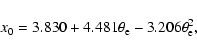
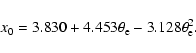
Using the general, exact relativistic approach discussed in this section, we evaluate the frequency location of the zero of the thermal SZ effect, x₀, for different cluster temperatures in the range 2-20 keV. The frequency location of x₀ depends on the IC gas temperature (or more generally on the IC gas pressure) and in Fig. 2 we compare the temperature dependence of x₀ evaluated at first order in $\tau$ (which actually does not depend on $\tau$) with that evaluated in the exact approach for values $\tau =10^{-3}$ and $\tau =10^{-2}$.

Figure 2: The location of x0 for a thermal electron population is shown as a function of $k_{\rm B}T_{\rm e}$. The exact calculation for $\tau =10^{-2}$ (solid line) and for $\tau =10^{-3}$ (dashed line) are shown together with the approximated calculation to first order in $\tau$ (dotted line).

 

 

Table 2: The fractional error $\varepsilon$ done considering the first, second and third order approximation in $\tau$ compared with the exact calculation of the thermal SZ effect is reported for three interesting values of the frequency x. The assumed values of $k_{\rm B}T_{\rm e}$ and $\tau$ are shown in the first column of the table. The values of $\varepsilon$ are given in units of 10^-2.

	First order	Second order	Third order
$k_{\rm B}T_{\rm e}=20$ keV
$\tau =10^{-2}$
x=2.3	0.31	0.22	0.22
x=6.5	0.12	0.27	0.27
x=15	2.23	1.71	1.71
$k_{\rm B}T_{\rm e}=20$ keV
$\tau =10^{-3}$
x=2.3	0.24	0.23	0.23
x=6.5	0.21	0.23	0.23
x=15	0.23	0.18	0.18
$k_{\rm B} T_{\rm e}=10$ keV
$\tau =10^{-2}$
x=2.3	0.02	0.02	0.02
x=6.5	0.7	0.02	0.02
x=15	0.74	0.21	0.21
$k_{\rm B} T_{\rm e}=10$ keV
$\tau =10^{-3}$
x=2.3	0.01	0.01	0.01
x=6.5	0.01	0.02	0.01
x=15	0.31	0.25	0.25

The location of the null of the SZ effect increases by $\sim$4.4% for $k_{\rm B}T_{\rm e}$ up to $\sim$20 keV. Assuming a quadratic fit $x_0 \approx a+b \theta_{\rm e} + c \theta_{\rm e}^2$, where $\theta _{\rm e}=k_{\rm B}T_{\rm e}/m_{\rm e}c^2$, we calculate the coefficients a, b and c which fit the temperature dependence of x₀. These are given in Table 3.

 

 

Table 3: The coefficients of the quadratic fit of the behaviour $x_{\rm0,th}$ as a function of $\theta _{\rm e}=k_{\rm B}T_{\rm e}/m_{\rm e}c^2$ (see text for details).

	a	b	c
Exact $\; \tau=0.001$	3.8271	4.6059	-4.8221
Exact $\; \tau=0.01$	3.8262	4.6704	-5.4895
First order	3.8294	4.4304	-1.7805

In particular the coefficients of the last row in Table 3 can be compared with those given by Itoh et al. (1998). At first order in $k_{\rm B}T_{\rm e}$, and for IC gas temperatures up to 50 keV, these last authors found $x_0 \approx 3.830+4.471\theta_{\rm e}-3.268\theta_{\rm e}^2$. The coefficients given in the first two rows of Table 3 can be also compared with those found by Dolgov et al. (2000), who gave the expression of x₀ evaluated in an exact way for a temperature range $0\leq k_{\rm B} T_{\rm e} \leq 50$ keV and for $0 \leq \tau \leq 0.05$: $x_0=\alpha(T_{\rm e})+\tau \beta(T_{\rm e})$ with $\alpha(T_{\rm e})= 3.830(1+1.162\theta_{\rm e} -0.8144\theta_{\rm e}^2)$ and $\beta(T_{\rm e})= 3.021\theta_{\rm e} -8.672\theta_{\rm e}^2$.

For $\tau =0.01$, the expression for x₀ derived by Dolgov et al. (2000) writes as

$$x_0=3.830+4.481\theta_{\rm e}-3.206\theta_{\rm e}^2,$$ (30)

while for $\tau =0.001$ one gets

$$x_0=3.830+4.453\theta_{\rm e}-3.128\theta_{\rm e}^2 .$$ (31)

The remaining differences with our coefficients given in Table 3 are due to the different $T_{\rm e}$ and $\tau$ ranges used for the quadratic fit.