Adopting the interpretation in terms of the plasma emission from
the upstream and downstream shock regions, the band-split
frequencies map the electron densities behind and ahead of the
shock front. In front of the shock (upstream region) the plasma is
characterized by the electron density n1 and emits radio waves
at the frequency ![]() (lower frequency branch; LFB). The
plasma behind the shock (downstream region) is compressed to the
density n2 > n1 corresponding to the frequency
(lower frequency branch; LFB). The
plasma behind the shock (downstream region) is compressed to the
density n2 > n1 corresponding to the frequency
![]() (upper frequency branch; UFB). Defining the relative
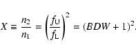
band-split (Fig. 1, see also Paper I) as:
(upper frequency branch; UFB). Defining the relative
band-split (Fig. 1, see also Paper I) as:
| (1) |
 |
(2) |
On the other hand, the emission frequency f can be transformed
into the radial distance r by assuming some density distribution
function n(r). Consequently, the shock propagation speed
![]() can be inferred from the frequency drift
can be inferred from the frequency drift
![]() ,
providing evaluation of the Alfvén
velocity
,
providing evaluation of the Alfvén
velocity
![]() .
Finally, the magnetic field can be found
using (m.k.s.):
.
Finally, the magnetic field can be found
using (m.k.s.):
![]() ,
where the coronal plasma density is approximated as
,
where the coronal plasma density is approximated as
![]() ,
and
,
and
![]() H m-1. A more practical
expression reads:
H m-1. A more practical
expression reads:
![\begin{displaymath}%
B~[{\rm gauss}]= 5.1\times 10^{-5}\times f~[{\rm MHz}]\times
v_{\rm A}~\left[{\rm km~s^{-1}}\right].
\end{displaymath}](/articles/aa/full/2002/47/aa2984/img44.gif) |
(3) |
The emission frequency depends on the local electron density which can be a complicated function of space coordinates, especially in active regions. We note that most of the measurements are performed at frequencies corresponding to relatively large heights, well outside of the active region core. Therefore we assume that the plasma density depends only on the height. In particular, the Saito (1970) and Newkirk (1961) density models with various base densities are applied (see Fig. 8 in Appendix).
Radioheliographic observations indicate that the type II burst
sources frequently do not propagate radially, especially at the
onset of the burst (see, e.g., Nelson & Robinson 1975;
Klassen et al. 1999; Klein et al. 1999). This means
that the shock velocity v' is generally underestimated if the
radial propagation is assumed. Accordingly, smaller values of the
Alfvén speed and the magnetic field are obtained. For a given
angle ![]() between the (radial) density gradient and the
direction of the source motion, the true source velocity is found
using
between the (radial) density gradient and the
direction of the source motion, the true source velocity is found
using
![]() .
Therefore, if
.
Therefore, if
![]() the
evaluation of true velocity is reduced to a simple multiplication
of the model densities by factor
the
evaluation of true velocity is reduced to a simple multiplication
of the model densities by factor
![]() .
For example, the
same speed is obtained by using the five-fold Saito density model
and
.
For example, the
same speed is obtained by using the five-fold Saito density model
and
![]() ,
or by applying the ten-fold Saito model and
,
or by applying the ten-fold Saito model and
![]() .
.
In a statistical sense the problem can be solved by introducing
the mean angle
![]() at which an "average source" moves
through an "average corona". Assuming that most often the corona
can be described by the two- to five-fold Saito model, we will
present also the outcome for the ten-fold Saito model with
at which an "average source" moves
through an "average corona". Assuming that most often the corona
can be described by the two- to five-fold Saito model, we will
present also the outcome for the ten-fold Saito model with
![]() to represent the propagation in the five-fold
Saito model corona under assumption of a strong,
to represent the propagation in the five-fold
Saito model corona under assumption of a strong,
![]() ,
deviation from the radial propagation.
,
deviation from the radial propagation.
The MHD relationship between the density jump and the Mach number
depends on the angle ![]() between the shock normal and the
magnetic field direction. In the quasi-perpendicular regime
between
between the shock normal and the
magnetic field direction. In the quasi-perpendicular regime
between
![]() and, say,
and, say,
![]() the
outcome is only weakly dependent on the value of
the
outcome is only weakly dependent on the value of ![]() (see Fig. 9a in Appendix). Comparing the longitudinal,
(see Fig. 9a in Appendix). Comparing the longitudinal,
![]() ,
and the perpendicular,
,
and the perpendicular,
![]() ,
propagation one finds that the calculated values of
,
propagation one finds that the calculated values of ![]() are
10-25% lower in the longitudinal case, the difference being
larger for a larger band-split.
are
10-25% lower in the longitudinal case, the difference being
larger for a larger band-split.
Another important parameter is the plasma-to-magnetic pressure
ratio
![]() in the upstream region (see Fig. 9b in Appendix). Highly structured patterns observed
in the EUV wavelength range indicate that the coronal plasma is
controlled by the magnetic field, i.e.,
in the upstream region (see Fig. 9b in Appendix). Highly structured patterns observed
in the EUV wavelength range indicate that the coronal plasma is
controlled by the magnetic field, i.e.,
![]() (for a discussion see Gary 2001). Since the relationship
(for a discussion see Gary 2001). Since the relationship
![]() only weakly depends on the value of
only weakly depends on the value of ![]() when it is
smaller than
when it is
smaller than ![]() 0.2 (see Fig. 9b in Appendix) we
apply
0.2 (see Fig. 9b in Appendix) we
apply ![]() .
This approximation will be checked finally: after
the B(r) dependence is established using some density model
n(r), the assumption
.
This approximation will be checked finally: after
the B(r) dependence is established using some density model
n(r), the assumption
![]() can be verified
taking for the coronal temperature T= 1-2
can be verified
taking for the coronal temperature T= 1-2
![]() K
(Chae et al. 2002).
K
(Chae et al. 2002).
In order to check how much various approximations affect the results, the analysis is carried out using several different values for all relevant parameters.
Copyright ESO 2002
![\begin{figure}
\par\includegraphics[width=14.5cm,clip]{MS2984f1.eps} \end{figure}](/articles/aa/full/2002/47/aa2984/img60.gif)