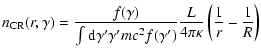
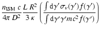
Based on the picture laid out in Sect. 3, we can try to predict what might be observed in the CR spectrum due to the presence of Galactic microquasars.
First, it is obvious that close enough to a powerful relativistic jet source the locally observed CR spectrum will be completely dominated by the CRs produced in the terminal shock of the jet. However, it is clear that the powerlaw spectrum observed near earth is not dominated by a narrow component of microquasar origin - the current spectral limits rule out any contribution greater than a few percent.
In a simple isotropic diffusion picture, the CR energy density in the
environment of a continuously active source will fall roughly like the
inverse distance to the source r-1 (see Eq. (8)) for
large r much larger than a particle mean free path,
![]() ,
and smaller than the Galactic disk
height,
,
and smaller than the Galactic disk
height,
![]() .
.
Given the observed CR energy density of ![]() 10
10
![]() ,
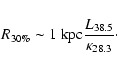
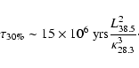
we can estimate that the sphere of influence of a given source,
defined as the region inside which the source contributes more than 30% of
the total measured CR power (at which level it would enter the
realm of detectability of by AMS 02) has a radius of order
,
we can estimate that the sphere of influence of a given source,
defined as the region inside which the source contributes more than 30% of
the total measured CR power (at which level it would enter the
realm of detectability of by AMS 02) has a radius of order
 |
(5) |
 |
(6) |
The well known microquasars mentioned above are all located much further
from the solar system than this limit. However, if a source similar to,
say, GRS 1915+105 had been active in the solar neighborhood (inside about 1
kpc) within the last ![]() 107 yrs, our local CR flux should show a
clear sign of the contribution from this source.
107 yrs, our local CR flux should show a
clear sign of the contribution from this source.
In this context it is important to mention that GRO J1655-40, V4641 Sgr, Cyg X-3 (and also SS433) are known to be in high-mass X-ray binaries. Their lifetimes are therefore expected to be short. If such a relativistic jet black hole binary was located in the Orion nebula region within the past 106 yrs, we should be able to detect a strong signal in the low energy CR spectrum from this source alone.
Far enough away from any single source, an observer will measure the time
averaged contribution from all Galactic sources, washed out by CR diffusion
(similar to the situation described in Strong & Moskalenko 2001). Since sources
will likely follow a distribution of Lorentz factors of width
![]() ,
the observed signal will be smeared out over at least
that width. Any intrinsic width of the produced CR spectrum will add to
this effect, as well as broadening effects like solar modulation and
scattering off of interstellar turbulence.
,
the observed signal will be smeared out over at least
that width. Any intrinsic width of the produced CR spectrum will add to
this effect, as well as broadening effects like solar modulation and
scattering off of interstellar turbulence.
In Fig. 7 we have plotted possible contributions to the
CR proton spectrum from a single Galactic jet source. Depending on how
much we have underestimated the power in Galactic jets and how much
adiabatic losses of particles trapped in adiabatically expanding shock will
suffer, we might over or underestimate the contribution. Taking the figure
at face value, however, it seems likely that a contribution at the few
percent level can be expected in the energy region of a few GeV.
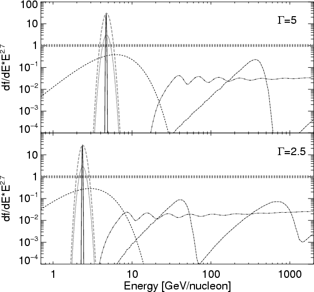 |
Figure 7:
Toy model of the microquasar contribution to the CR spectrum, for
a single microquasar situated in a low mass X-ray binary, active for
|
For an effective area of order
![]() ,
the expected total CR
proton count rate by AMS 02 in the energy range from 1 to 10 GeV
should be of the order of
,
the expected total CR
proton count rate by AMS 02 in the energy range from 1 to 10 GeV
should be of the order of
![]() .
At 2% energy
resolution, this implies a detection rate of about
.
At 2% energy
resolution, this implies a detection rate of about
![]() ,
with a relative Poisson-noise level of order
10-4. Calibration and other systematic errors will likely dominate
the statistics, however, these numbers are encouraging, and we expect that
a source at the few-percent level will be detectable with AMS 02.
,
with a relative Poisson-noise level of order
10-4. Calibration and other systematic errors will likely dominate
the statistics, however, these numbers are encouraging, and we expect that
a source at the few-percent level will be detectable with AMS 02.
The heavy element sensitivity of AMS 02 will share similar
characteristics: for the same energy resolution and effective area, the
detection rates of carbon and iron, for example, should be of order
![]() and
and
![]() respectively. Aside from AMS 02, signatures might
be detected by other instruments, and even existing data sets might contain
signals. Identification would require scanning these data with high
spectral resolution. Note that the effects of solar modulation will
broaden any narrow spectral component significantly. Results by
Labrador & Mewaldt (1997) demonstrate that a line at
respectively. Aside from AMS 02, signatures might
be detected by other instruments, and even existing data sets might contain
signals. Identification would require scanning these data with high
spectral resolution. Note that the effects of solar modulation will
broaden any narrow spectral component significantly. Results by
Labrador & Mewaldt (1997) demonstrate that a line at ![]() 5 GeV will
be broadened by
5 GeV will
be broadened by ![]() 1 GeV, (less at higher energies) though this
effect will be reduced at solar minimum.
1 GeV, (less at higher energies) though this
effect will be reduced at solar minimum.
As the CRs produced in microquasars travel traverse the Galaxy, they will
encounter the cold ISM. The interaction of a CR proton (by far the most
abundant and thus most energetic component of the CR spectrum) with a cold
ISM proton can lead to secondary particle production and to the emission of
gamma rays via several channels, the most important of which is ![]() decay.
decay.
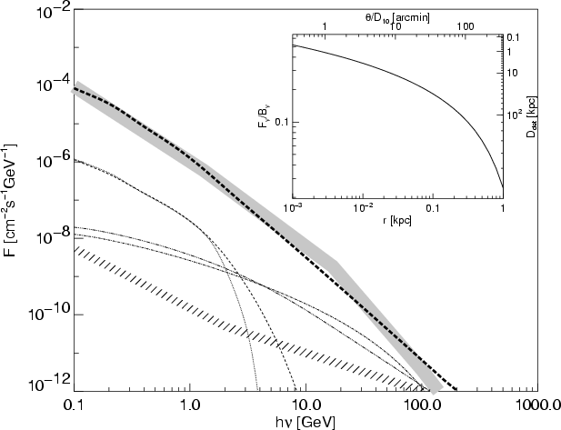 |
Figure 8:
Toy model for the gamma ray signature produced in a microquasar
CR halo via pion decay (including |
Using the toy model presented in Fig. 7, we can estimate
how much gamma ray flux can be expected from the CR halo of a powerful
microquasar and compare it to the background flux from the Galaxy. We
assume that the CRs diffuse away from the source until they reach the
Galactic halo, approximated as a zero pressure boundary condition at radius
![]() (assuming spherical
symmetry for simplicity). The result is shown in
Fig. 8.
(assuming spherical
symmetry for simplicity). The result is shown in
Fig. 8.
Note that the gamma ray signal even for a source of average kinetic power
of
![]() is small compared to
the background signal coming from the same solid angle (
is small compared to
the background signal coming from the same solid angle (![]() ).
However, because the CR density increases towards the center of the source,
higher spatial resolution can improve the signal-to-noise ratio somewhat.
For a spherically symmetric cloud of CRs with luminosity L and vanishing
pressure at the boundary
).
However, because the CR density increases towards the center of the source,
higher spatial resolution can improve the signal-to-noise ratio somewhat.
For a spherically symmetric cloud of CRs with luminosity L and vanishing
pressure at the boundary
![]() ,
the density follows
,
the density follows
However, they could act as a significant ionization source for the
surrounding medium: the ionization loss timescale for a particle with
energy
![]() is of order (Ginzburg 1979)
is of order (Ginzburg 1979)
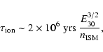 |
(9) |
Furthermore, the excitation of nuclear ![]() -ray emission lines by
interaction of these sub-cosmic rays with interstellar heavy ions of C, O,
Fe, and other elements might be detectable by INTEGRAL.
-ray emission lines by
interaction of these sub-cosmic rays with interstellar heavy ions of C, O,
Fe, and other elements might be detectable by INTEGRAL.
If the jet consists chiefly of relatively cold electron-positron plasma, and
if dissipation occurs mostly in the reverse shock, then the jet terminus
will produce relativistic electrons and positrons with energies of the
order of
![]() ,
which will
then begin to diffuse into the ISM. Such positrons and electrons could
produce additional bremsstrahlung radiation at energies of a few hundreds of
keVs up to 2.5 MeV. Much like mildly relativistic protons, these electrons
will contribute to the heating of the ISM due to the ionization losses, but
much more important for future observations might be the
electron-positron annihilation line at 511 keV.
,
which will
then begin to diffuse into the ISM. Such positrons and electrons could
produce additional bremsstrahlung radiation at energies of a few hundreds of
keVs up to 2.5 MeV. Much like mildly relativistic protons, these electrons
will contribute to the heating of the ISM due to the ionization losses, but
much more important for future observations might be the
electron-positron annihilation line at 511 keV.
For an integrated mechanical luminosity of
![]() of the entire ensemble of Galactic
relativistic jets, the flux of positrons carried by jets is
of the entire ensemble of Galactic
relativistic jets, the flux of positrons carried by jets is
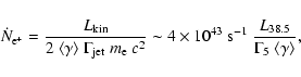 |
(10) |
This is actually comparable to the total amount of positrons annihilating
in the Galaxy according to the observations of the e+/e-annihilation line from OSSE/GRO,
![]() (Purcell et al. 1997). If Galactic jets are in
fact composed of electron-positron plasma, this measurement immediately
implies one of the following conclusions: a) either the mechanical
luminosity of these jets is not far above our relatively conservative
estimate of
(Purcell et al. 1997). If Galactic jets are in
fact composed of electron-positron plasma, this measurement immediately
implies one of the following conclusions: a) either the mechanical
luminosity of these jets is not far above our relatively conservative
estimate of
![]() ,
or b) the pair
plasma is not cold, i.e.,
,
or b) the pair
plasma is not cold, i.e.,
![]() ,
or c)
diffusion of particles across the magnetic boundary of the remnant jet
plasma is very inefficient, in which case many Galactic "radio relics''
should exist, not unlike in the case of radio relics from radio loud AGNs
in the intracluster medium (e.g., Ensslin et al. 1998).
,
or c)
diffusion of particles across the magnetic boundary of the remnant jet
plasma is very inefficient, in which case many Galactic "radio relics''
should exist, not unlike in the case of radio relics from radio loud AGNs
in the intracluster medium (e.g., Ensslin et al. 1998).
The Integral SPI spectrometer and the IBIS imager would be able to measure the increase in the annihilation line flux towards microquasars located away from the Galactic center (where the background is highest) like GRS1915+105, and to measure the line width if it could be detected. These measurements could be very helpful in constraining the particle content of relativistic Galactic jets.
Copyright ESO 2002