The non-LTE spectrum formation is calculated for an expanding atmosphere under the standard assumptions of spherical symmetry, stationarity and homogeneity. The model calculations are in line with our previous work (Koesterke et al. 1992; Hamann et al. 1992; Koesterke & Hamann 1995; Leuenhagen & Hamann 1994; Leuenhagen et al. 1996; Hamann & Koesterke 1998). However, for the inclusion of iron group line-blanketing we had to modify our code extensively. In this section, we give a summarizing description of the method with special emphasize to those new features which concern the iron line-blanketing.
A model atmosphere is specified by the luminosity and radius of the stellar core at the inner
boundary, and by the chemical composition and the density- and velocity structure of the
envelope. For the stellar core the radius ![]() at Rosseland optical depth
at Rosseland optical depth
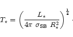
![]() and the stellar temperature
and the stellar temperature ![]() are prescribed.
are prescribed. ![]() is related to the
stellar luminosity
is related to the
stellar luminosity ![]() by Stefan-Boltzmann's law
by Stefan-Boltzmann's law
| Ion | Levels | Ion | Super-levels | Sub-levels | |
| He I | 17 | Fe III | 1 | ||
| He II | 16 | Fe IV | 18 | 30 122 | |
| He III | 1 | Fe V | 19 | 19 804 | |
| C I | 2 | Fe VI | 18 | 15 155 | |
| C II | 32 | Fe VII | 16 | 11 867 | |
| C III | 40 | Fe VIII | 10 | 8669 | |
| C IV | 54 | Fe IX | 11 | 12 366 | |
| C V | 1 | Fe X | 1 | ||
| O II | 3 | ||||
| O III | 33 | ||||
| O IV | 25 | ||||
| O V | 36 | ||||
| O VI | 15 | ||||
| O VII | 1 | ||||
| Si III | 10 | ||||
| Si IV | 7 | ||||
| Si V | 1 |
Density-inhomogeneities (clumping) are accounted for in the limit of small-scale clumps with a
density enhanced by a factor D = 1/fV over the mean density ![]() (see Schmutz 1995; Hillier 1996; Hamann & Koesterke 1998). The inter-clump medium is supposed to be void. The
radiation transport is calculated for the spatially averaged opacity, whereas the statistical
equations are solved for the enhanced density in the clumps.
(see Schmutz 1995; Hillier 1996; Hamann & Koesterke 1998). The inter-clump medium is supposed to be void. The
radiation transport is calculated for the spatially averaged opacity, whereas the statistical
equations are solved for the enhanced density in the clumps.
For models with the same stellar temperature ![]() ,
the strength of emission lines depends
mainly on the so-called transformed radius
,
the strength of emission lines depends
mainly on the so-called transformed radius ![]() ,
which is defined as
,
which is defined as
The chemical composition is given by mass fractions
![]() ,
,
![]() ,
,
![]() ,
,
![]() and
and
![]() of helium, carbon, oxygen, silicon and iron group elements. The
model atoms contain the ionization stages He I-He III, C I-C V, O II-O VII, Si III-Si V and Fe III-Fe X. Except for He I and Si III, the lowest
and highest ionization stages are restricted to a few auxiliary levels. A summarizing
description of the model atoms is given in Table 1.
of helium, carbon, oxygen, silicon and iron group elements. The
model atoms contain the ionization stages He I-He III, C I-C V, O II-O VII, Si III-Si V and Fe III-Fe X. Except for He I and Si III, the lowest
and highest ionization stages are restricted to a few auxiliary levels. A summarizing
description of the model atoms is given in Table 1.
Due to the iron group elements, almost the whole spectral range is crowded by lines. Therefore, we abandon the distinction between continuum- and spectral line transfer used in our previous code. Analogous to the work of Hillier & Miller (1998), the radiation transfer is now calculated on one comprehensive frequency grid, which covers the whole relevant frequency range with typically three points per Doppler width wherever line opacities are present, and a wider spacing in pure-continuum regions.
The equation of radiative transfer in a spherically-expanding atmosphere is formulated in the
co-moving frame of reference, neglecting aberration and advection terms (Mihalas et al. 1976a). The
angle dependent transfer equation then becomes a partial differential equation for the
intensity ![]() ,
,
In the present work, the numerical solution of Eq. (4) is achieved by a
short-characteristic method, described in detail in Koesterke et al. (2002). However, as the
angle-dependent equation is computationally expensive, and because of the drawback with the
Thomson-scattering term, we employ the "method of variable Eddington factors''
(Auer & Mihalas 1970). This means, the angle-dependent transfer equation is only solved from time to
time (typically every six ALI iteration cycles). The resulting intensities ![]() at each
radius and frequency grid point are integrated up over angles with weight factors
at each
radius and frequency grid point are integrated up over angles with weight factors ![]() ,
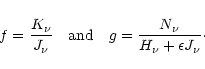
yielding the nth moments of the radiation field J, H, K and N for n = 0, 1, 2 and
3, respectively. Only the Eddington factors f and g are finally exploited from that step,
which are defined as
,
yielding the nth moments of the radiation field J, H, K and N for n = 0, 1, 2 and
3, respectively. Only the Eddington factors f and g are finally exploited from that step,
which are defined as
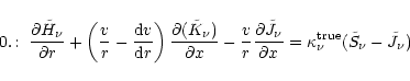
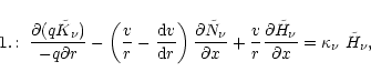
Based on these Eddington factors, the radiative transfer is solved in each ALI iteration cycle
by means of the moment equations. By integration of Eq. (4) over ![]() (weighted with
(weighted with ![]() and
and ![]() respectively), one obtains the zeroth and first moment
equation as
respectively), one obtains the zeroth and first moment
equation as
After the moments ![]() and
and ![]() are substituted in Eqs. (6) and (7) with the help of the Eddington factors (Eq. (5)), these are
solved by a differencing scheme as proposed by Mihalas et al. (1976b).
are substituted in Eqs. (6) and (7) with the help of the Eddington factors (Eq. (5)), these are
solved by a differencing scheme as proposed by Mihalas et al. (1976b).
In the ALI formalism, the consistent solution of the equations of statistical equilibrium and the radiative transfer equation is achieved iteratively by solving both sets of equations in turn. However, in order to obtain convergence it is necessary to "accelerate'' the iteration by incorporating some "approximate'' radiative transfer into the statistical equation, which at least accounts for the locally trapped radiation in optically thick situations.
In the present work we use the concept of Hamann (1985, 1986). However, our definition of the diagonal "approximate lambda operators'' must be modified and extended with respect to the iron-line opacities, as we will describe in the following.
As in Hamann (1986), the atomic population numbers ![]() are calculated at each depth
point from the equations of statistical equilibrium, which are of the form
are calculated at each depth
point from the equations of statistical equilibrium, which are of the form
 |
(8) |
This set of nonlinear equations is solved numerically by the application of a hybrid technique,
a combination of the Broyden and the Newton algorithm (Hamann 1987; Koesterke et al. 1992). For this
purpose the Jacobian matrix
![]() must be calculated
occasionally, and the derivatives
must be calculated
occasionally, and the derivatives
![]() must be provided for
all relevant transitions.
must be provided for
all relevant transitions.
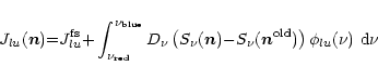
The calculation of the
![]() and their derivatives is modified in
comparison to Hamann (1985). For line transitions we keep the core saturation approach but
utilize the "diagonal operator'' of Rybicki & Hummer (1991) for the core integration, additionally
accounting for the interaction with blending iron opacities. The continuum and iron
transition rates are also calculated using the diagonal operator but in the "standard''
approach, i.e. the full frequency integral is performed (see Sect. 3.3
for iron transitions).
and their derivatives is modified in
comparison to Hamann (1985). For line transitions we keep the core saturation approach but
utilize the "diagonal operator'' of Rybicki & Hummer (1991) for the core integration, additionally
accounting for the interaction with blending iron opacities. The continuum and iron
transition rates are also calculated using the diagonal operator but in the "standard''
approach, i.e. the full frequency integral is performed (see Sect. 3.3
for iron transitions).
The diagonal operator provides the local response of the radiation field on the population numbers as a by-product of the radiative transfer. By applying it to the discretized moment Eqs. (6) and (7), we obtain the response on the true source function, fully accounting for coherent scattering.
In discretized form ![]() is represented by a vector
is represented by a vector ![]() on the radial depth grid
at the corresponding frequency index k, and the first moment vector
on the radial depth grid
at the corresponding frequency index k, and the first moment vector ![]() is defined on
the radius interstices. After elimination of
is defined on
the radius interstices. After elimination of ![]() by substitution of
Eq. (7) into Eq. (6) one obtains a second order equation of the
form
by substitution of
Eq. (7) into Eq. (6) one obtains a second order equation of the
form
At this point it is possible to extract the diagonal
![]() ,
which describes the local response of the radiation field on the
source function, i.e.
,
which describes the local response of the radiation field on the
source function, i.e.
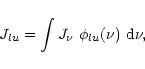
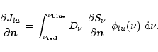
For a line transition between the energy levels l and u, the radiation field enters the
radiative rates via the scattering integral
The derivatives
![]() are calculated directly from
Eq. (12)
are calculated directly from
Eq. (12)
 |
(13) |
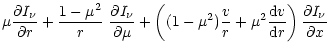
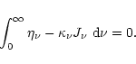
The temperature stratification has to be derived from the equation of radiative equilibrium in
the co-moving frame
A sufficient model accuracy is reached when the correction between consecutive ALI iterations drops below 1%. The convergence properties depend strongly on the start model. In practice it is often possible to choose start models which are already close to the solution. In such a case about 40 iterations are needed to obtain convergence. For a model which is started from LTE, this number can increase by a factor of 10. In the case of the line blanketed WC model in Sect. 4 (70 depth points, 396 levels, 36 210 frequencies) 24 iterations are needed from a "good'' start model, whereas 300 iterations are necessary for an LTE start. The computing time per ALI iteration cycle ranges from 150 to 350 s on a Compaq Alpha XP1000/667 workstation.
Copyright ESO 2002
![\begin{displaymath}%
R_{\rm t} = R_\star \left[\frac{v_\infty}{2500 ~ {\rm km}~{...
...10^{-4} ~ {M_\odot}~{\rm yr^{-1}}}\right]^{2/3}
\right. \cdot
\end{displaymath}](/articles/aa/full/2002/19/aah3177/img30.gif)