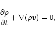
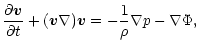
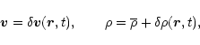
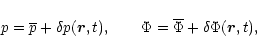
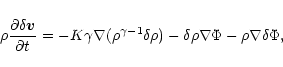
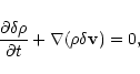
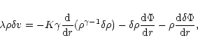
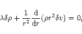
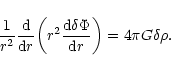
We shall now investigate the dynamical stability of polytropic gas spheres against radial perturbations. We use a method and presentation similar to that adopted for isothermal spheres in Chavanis (2002a). The equations describing the motions of a gaseous star are the equation of continuity, the Euler equation and the Poisson equation
 ,
,
 ,..., the equations of the problem become
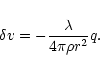
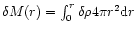 within the sphere of radius r. Thus, by definition, q(0)=0. Then, it is readily seen that the Poisson equation (44) is equivalent to
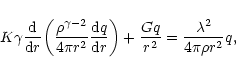
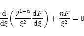
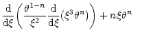
Considering the case of marginal stability  and introducing the dimensionless variables defined in Sect. 2, we can reduce the equation of radial pulsations to the form
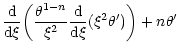
 the differential operator appearing in Eq. (50) and using the Lane-Emden Eq. (7), we easily establish that
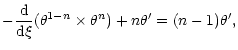
 and
and
 .
.
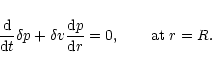
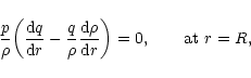
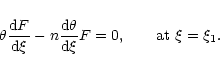
The equation of pulsations (49) must be supplemented by appropriate boundary conditions. For self-confined polytropes (1<n<5), we require that the Lagrangian derivative of the pressure vanishes at the surface of the configuration, i.e.
 ,
this yields n=3. Therefore, the transition from stability to instability occurs for a polytropic index n=3 or, equivalently, for an adiabatic index
,
this yields n=3. Therefore, the transition from stability to instability occurs for a polytropic index n=3 or, equivalently, for an adiabatic index
 .
Of course, this result is well-known and could have been obtained from the general theorems of stellar pulsation (see, e.g., Cox 1980). However, we provide here an alternative method based on the explicit resolution of the equation of pulsations for polytropes.
.
Of course, this result is well-known and could have been obtained from the general theorems of stellar pulsation (see, e.g., Cox 1980). However, we provide here an alternative method based on the explicit resolution of the equation of pulsations for polytropes.
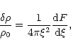
According to Eq. (45), the perturbation profile at the point of marginal stability is given by
 .
Simplifying the derivative with the aid of the Lane-Emden Eq. (7), we obtain
.
Simplifying the derivative with the aid of the Lane-Emden Eq. (7), we obtain
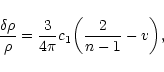
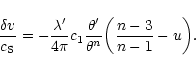
 On the other hand, the velocity profile is
given by Eq. (47). Normalizing with a typical velocity
On the other hand, the velocity profile is
given by Eq. (47). Normalizing with a typical velocity
 ,
we find that
,
we find that
 so that Eq. (60) is applicable with
 .
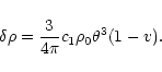
Substituting explicitly for n=3, we get
.
Substituting explicitly for n=3, we get
For polytropes confined within a box, the boundary condition consistent with the conservation of mass is
 .
With the expression (53) for ,
this yields
.
With the expression (53) for ,
this yields
 is monotonous. For
 ,
the configurations with
,
the configurations with
 are unstable but there are no secondary instabilities. For n>5, a first mode of stability is lost for
 .
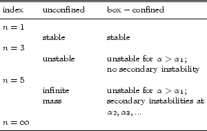
Subsequent oscillations in the mass-density profile are associated with secondary instabilities. A summary of the stability limits for polytropic gas spheres is given in Table 1. In Fig. 7 we have plotted the density contrast at the critical point
as a function of the index of the polytrope. For
.
Subsequent oscillations in the mass-density profile are associated with secondary instabilities. A summary of the stability limits for polytropic gas spheres is given in Table 1. In Fig. 7 we have plotted the density contrast at the critical point
as a function of the index of the polytrope. For  ,
the polytropes are stable and
,
the polytropes are stable and
 .
For n>3, only configurations with a density contrast
.
For n>3, only configurations with a density contrast
 are stable. For
 ,
the critical density contrast tends to its classical value
,
the critical density contrast tends to its classical value
 (see Chavanis 2002a).
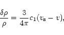
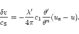
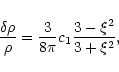
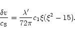
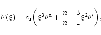
Using Eqs. (58), (60), the profiles of density and velocity that trigger the instabilities at the critical points can be written
 for the mode of instability of order k. We can determine the qualitative behavior of these profiles graphically by considering the intersections between the solution curve in the (u,v) plane and the lines
 and
and
 (see Figs. 2-4). These intersections determine the nodes of the perturbation profile. For
,
there is only one intersection since the (u,v) curve is monotonous. For n=5, we obtain the analytical solutions
(see Figs. 2-4). These intersections determine the nodes of the perturbation profile. For
,
there is only one intersection since the (u,v) curve is monotonous. For n=5, we obtain the analytical solutions
 has its node at
 .
For n>5, there are several intersections with the spiral since the lines
and
pass through the fixed point. The description of the perturbation profiles is similar to the one given for isothermal spheres (
.
For n>5, there are several intersections with the spiral since the lines
and
pass through the fixed point. The description of the perturbation profiles is similar to the one given for isothermal spheres ( ). The density profile of the fundamental mode of instability (at
)
has only one node. High order modes of instability (at
). The density profile of the fundamental mode of instability (at
)
has only one node. High order modes of instability (at
 ,
k>1) present numerous oscillations whose nodes asymptotically follow a geometric progression. We refer to our previous paper (Chavanis 2002a) for a more precise description of these results.
,
k>1) present numerous oscillations whose nodes asymptotically follow a geometric progression. We refer to our previous paper (Chavanis 2002a) for a more precise description of these results.
Copyright ESO 2002









![\begin{figure}
\par\includegraphics[width=8.8cm,clip]{deltarho3P.eps}\end{figure}](/articles/aa/full/2002/17/aa1920/img142.gif)

![\begin{figure}
\par\includegraphics[width=8.8cm,clip]{ncontrastP.eps}\end{figure}](/articles/aa/full/2002/17/aa1920/img150.gif)