

Up: Gravitational instability of polytropic
Subsections
2 Properties of polytropic gas spheres
2.1 The Lane-Emden equation
Polytropic stars are characterized by an equation of state of the form
 |
(1) |
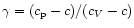
where K and  are constants. The index n of the polytrope is defined by the relation
 |
(2) |
The equation of state (1) corresponds to an adiabatic equilibrium in regions where convection keeps the star stirred up and produces a uniform entropy distribution (
 ). In that case,
is the ratio of specific heats
cp/cV at constant pressure and volume. For a monoatomic gas,
). In that case,
is the ratio of specific heats
cp/cV at constant pressure and volume. For a monoatomic gas,
 .
The equation of state (1) also describes a polytropic equilibrium characterized by a uniform specific heat
.
The equation of state (1) also describes a polytropic equilibrium characterized by a uniform specific heat
 .
In this more general situation
.
In this more general situation
 .
Convective equilibrium is recovered for c=0 and isothermal equilibrium is obtained in the limit of infinite specific heat
.
Convective equilibrium is recovered for c=0 and isothermal equilibrium is obtained in the limit of infinite specific heat
 .
A power law relation between the pressure and the density is also the limiting form of the equation of state describing a gas of cold degenerate fermions (Chandrasekhar 1932). In that case, the constant K can be expressed in terms of fundamental constants. In the classical limit
,
n=3/2 and
.
A power law relation between the pressure and the density is also the limiting form of the equation of state describing a gas of cold degenerate fermions (Chandrasekhar 1932). In that case, the constant K can be expressed in terms of fundamental constants. In the classical limit
,
n=3/2 and
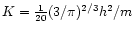 (where h is the Planck constant) and in the relativistic limit
 ,
n=3 and
,
n=3 and
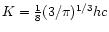 (where c is the speed of light). Historically, the index
appears in the classical theory of white dwarf stars initiated by Fowler (1926) and the index
is related to the limiting mass of Chandrasekhar (1931).
(where c is the speed of light). Historically, the index
appears in the classical theory of white dwarf stars initiated by Fowler (1926) and the index
is related to the limiting mass of Chandrasekhar (1931).
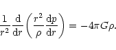
The condition of hydrostatic equilibrium for a spherically symmetrical distribution of matter reads
 |
(3) |
where  is the gravitational potential. Using the Gauss theorem
 |
(4) |
where
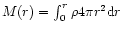 is the mass contained within the sphere of radius r, we can derive the fundamental equation of equilibrium (Chandrasekhar 1932)
 |
(5) |
Equations (1), (5) fully determine the structure of polytropic gas spheres. Letting
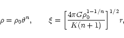 |
(6) |
where  is the central density, we can reduce the condition of hydrostatic equilibrium to the Lane-Emden equation (Chandrasekhar 1932)
 |
(7) |
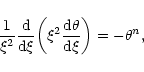
with boundary conditions
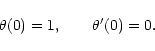 |
(8) |
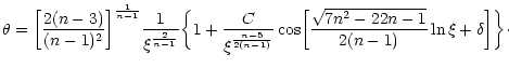
For n>3, the Lane-Emden equation admits an analytical solution which is singular at the origin:
 |
(9) |
Regular solutions of the Lane-Emden equation must in general be computed numerically. For
 ,
we can expand the function
,
we can expand the function  in Taylor series. The first terms in this expansion are given by
 |
(10) |
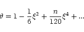
The behavior of
 at large distances deserves a more
specific discussion. For 1<n<5, the density falls off to zero at a
finite radius R, identified as the radius of the star. If we denote
by
at large distances deserves a more
specific discussion. For 1<n<5, the density falls off to zero at a
finite radius R, identified as the radius of the star. If we denote
by  the value of the normalized distance at which
  then, for
 ,
we have
,
we have
 |
(11) |
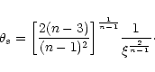
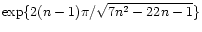
For n>5, the polytropes extend to infinity, like the isothermal configurations recovered in the limit  .
For
.
For
 ,
,
 |
|
|
(12) |
The curve (12) intersects the singular solution (9)
infinitely often at points that asymptotically increase geometrically
in the ratio 1:
 .
Since
.
Since
 at large distances, these
configurations have an "infinite mass'', which is clearly
unphysical. In the following, we shall restrict these configurations to a
"box'' of radius R, as in the classical Antonov
problem. Therefore, Eq. (7) must be solved for
at large distances, these
configurations have an "infinite mass'', which is clearly
unphysical. In the following, we shall restrict these configurations to a
"box'' of radius R, as in the classical Antonov
problem. Therefore, Eq. (7) must be solved for
 with
with
 |
(13) |
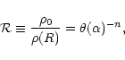
Note that, for a fixed box radius R,  is a measure of the central density .
The case n=5 is special. For this index, the Lane-Emden equation can be solved analytically and yields the result:
is a measure of the central density .
The case n=5 is special. For this index, the Lane-Emden equation can be solved analytically and yields the result:
 |
(14) |
The total mass of this configuration is finite but its potential energy diverges. Therefore, this polytrope must also be confined within a box. In Fig. 1, we have plotted different density profiles with index n=3,5,6.
![\begin{figure}
\par\includegraphics[width=8.8cm,clip]{profilesP.eps}\end{figure}](/articles/aa/full/2002/17/aa1920/Timg40.gif) |
Figure 1:
Density profiles of polytropes with index n=3,5,6. The dashed line corresponds to the singular solution (9). |
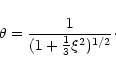
2.2 The Milne variables
As in the analysis of isothermal gas spheres, it will be convenient in the following to introduce the Milne variables (u,v) defined by (Chandrasekhar 1932):
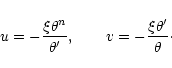 |
(15) |
Taking the logarithmic derivative of u and v with respect to  and using Eq. (7), we get
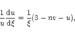 |
(16) |
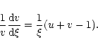 |
(17) |
Due to the homology invariance of the polytropic configuations (see Chandrasekhar 1932), the Milne variables u and v satisfy a first order differential equation
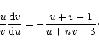 |
(18) |
The solution curve in the (u,v) plane (see Figs. 2-4) is parametrized by .
It starts from the point
(u,v)=(3,0) with a slope
 as
.
For 1<n<5, the curve is monotonous and tends to
as
.
For 1<n<5, the curve is monotonous and tends to
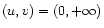 as
.
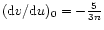
More precisely, using Eq. (11), we have
as
.
More precisely, using Eq. (11), we have
 |
(19) |
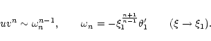
For n>5, the solution curve spirals indefinitely around the fixed point
 ,
corresponding to the singular solution (9), as
tends to infinity. All polytropic spheres must necessarily lie on this curve. For bounded polytropic spheres,
must be terminated at the box radius .
For n=5, the Milne variables are related according to
,
corresponding to the singular solution (9), as
tends to infinity. All polytropic spheres must necessarily lie on this curve. For bounded polytropic spheres,
must be terminated at the box radius .
For n=5, the Milne variables are related according to
![\begin{figure}
\par\includegraphics[width=8.8cm,clip]{uv4P.eps}\end{figure}](/articles/aa/full/2002/17/aa1920/Timg50.gif) |
Figure 2:
The (u,v) plane for polytropes with index 1<n<5. The construction is made explicitly for n=4. |
![\begin{figure}
\par\includegraphics[width=8.8cm,clip]{uv5P.eps}\end{figure}](/articles/aa/full/2002/17/aa1920/Timg51.gif) |
Figure 3:
The (u,v) plane for polytropes with index n=5. |
![\begin{figure}
\par\includegraphics[width=8.8cm,clip]{uv6P.eps}\end{figure}](/articles/aa/full/2002/17/aa1920/Timg52.gif) |
Figure 4:
The (u,v) plane for polytropes with index n>5. The construction is made explicitly for n=6. |
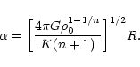
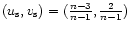
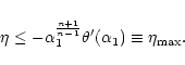
2.3 The maximum mass and minimum temperature of confined polytropes
For polytropes confined within a box of radius R, there exists a well-defined relation between the mass M of the configuration and the central density
(through the parameter ). Starting from the relation
 |
|
|
(21) |
and using the Lane-Emden Eq. (7), we get
 |
(22) |
Expressing the central density in terms of ,
using Eq. (13), we obtain after some rearrangements
 |
(23) |
Introducing the parameter
 |
(24) |
the foregoing relation can be rewritten
 |
(25) |
For n<5, the normalized box radius
in necessarily
restricted by the inequality
 .
For the limiting
value
.
For the limiting
value
 ,
corresponding to an isolated polytrope satisfying
,
corresponding to an isolated polytrope satisfying
 ,
we have
,
we have
 |
(26) |
The quantity
 ,
defined by Eq. (19), has been tabulated by
Chandrasekhar (1932). The definition (24) of
,
defined by Eq. (19), has been tabulated by
Chandrasekhar (1932). The definition (24) of  and the
relation (25) between
and
are consistent with
the formulae derived in the case of an isothermal gas (see
Chavanis 2002a). This connexion is particularly relevant if we interpret
the constant K as a polytropic temperature
and the
relation (25) between
and
are consistent with
the formulae derived in the case of an isothermal gas (see
Chavanis 2002a). This connexion is particularly relevant if we interpret
the constant K as a polytropic temperature
 (see
Chandrasekhar 1932, p. 86). For
(see
Chandrasekhar 1932, p. 86). For
 ,
,
 and the parameter
reduces to the corresponding one for isothermal spheres
(
and the parameter
reduces to the corresponding one for isothermal spheres
(
 ,
,
 ,
,
 ).
).
![\begin{figure}\par\includegraphics[width=8.8cm]{alphaetaP.eps}\end{figure}](/articles/aa/full/2002/17/aa1920/Timg70.gif) |
Figure 5:
Mass-density profiles for polytropic configurations with index
n=2,3,4,5,6. A mass peak appears for the first time for the critical index n=3. |
The function
 is represented in Fig. 5 for
different values of the polytropic index n. Instead of ,
we could have used the density contrast
is represented in Fig. 5 for
different values of the polytropic index n. Instead of ,
we could have used the density contrast
 |
(27) |
which also provides a relevant parametrization of the solutions.
Using the Lane-Emden Eq. (7) and the definition of the
Milne variables (15), it is straightforward to check that the
condition of extremum
 is equivalent to
 |
(28) |
where, by definition,
 and
and
 refers to the singular solution (9). For
 ,
we recover the condition u0=1 previously derived for isothermal configurations (Chavanis 2002a). The values of
for which
is extremum are given by the intersection(s) between the solution curve in the (u,v) plane and the line u=us (see Figs. 2-4). For 1<n<3,
,
we recover the condition u0=1 previously derived for isothermal configurations (Chavanis 2002a). The values of
for which
is extremum are given by the intersection(s) between the solution curve in the (u,v) plane and the line u=us (see Figs. 2-4). For 1<n<3,
 and there is no intersection. The mass-density relation is therefore monotonous. For
 ,
the curve
presents a single maximum at
,
the curve
presents a single maximum at
 .
For n=3, this maximum is reached at the extremity of the curve (
.
For n=3, this maximum is reached at the extremity of the curve (
 ). For n=5,
 and the function
is explicitly given by
and the function
is explicitly given by
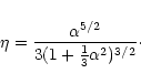 |
(29) |
The maximum of
is located at
 .
Finally, for n>5, the mass-density relation presents an infinite number of damped oscillations since the line defined by Eq. (28) passes through the center of the spiral in the (u,v) plane. If we denote by
.
Finally, for n>5, the mass-density relation presents an infinite number of damped oscillations since the line defined by Eq. (28) passes through the center of the spiral in the (u,v) plane. If we denote by
 the locii of the extrema of
,
these values asymptotically follow the geometric
progression
the locii of the extrema of
,
these values asymptotically follow the geometric
progression
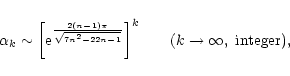 |
(30) |
obtained by substituting the asymptotic expansion (12) in Eq. (28). For
,
we recover the ratio
 corresponding to classical isothermal configurations (Semelin et al. 1999; Chavanis 2002a).
From the above results, it is clear that restricted polytropic spheres with index  can exist only for
 |
(31) |
This implies in particular the existence of a limiting mass (for a given confining radius R) such that
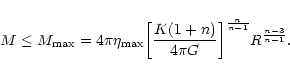 |
(32) |
For ,
we recover the limiting mass
 above which an isothermal sphere cannot sustain self-gravity (see, e.g., Chavanis 2002b). Alternatively, for a given mass M and radius R, the inequality (31) implies the existence of a minimum value of the polytropic temperature
 .
Indeed,
is restricted by the inequality
.
Indeed,
is restricted by the inequality
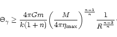 |
(33) |
In the limit ,
we recover the critical temperature
 below which an isothermal sphere is expected to collapse (Lynden-Bell & Wood 1968). This critical point, corresponding to
,
appears for the first time for the index n=3. This observation will take a deeper physical significance in the stability analysis performed in the following section. For
below which an isothermal sphere is expected to collapse (Lynden-Bell & Wood 1968). This critical point, corresponding to
,
appears for the first time for the index n=3. This observation will take a deeper physical significance in the stability analysis performed in the following section. For  ,
the mass-density profile is monotonous and
,
the mass-density profile is monotonous and
 .
The total mass (resp. temperature) of confined polytropes is always smaller (resp. larger) than the corresponding one for isolated polytropes. However, this bound does not correspond to a condition of extremum
but rather to the impossibility of constructing polytropes with
.
The total mass (resp. temperature) of confined polytropes is always smaller (resp. larger) than the corresponding one for isolated polytropes. However, this bound does not correspond to a condition of extremum
but rather to the impossibility of constructing polytropes with
 (since
can become negative).
(since
can become negative).
Up: Gravitational instability of polytropic
Copyright ESO 2002
![\begin{figure}
\par\includegraphics[width=8.8cm,clip]{profilesP.eps}\end{figure}](/articles/aa/full/2002/17/aa1920/img40.gif)
![\begin{figure}
\par\includegraphics[width=8.8cm,clip]{uv4P.eps}\end{figure}](/articles/aa/full/2002/17/aa1920/img50.gif)
![\begin{figure}
\par\includegraphics[width=8.8cm,clip]{uv6P.eps}\end{figure}](/articles/aa/full/2002/17/aa1920/img52.gif)
![\begin{figure}\par\includegraphics[width=8.8cm]{alphaetaP.eps}\end{figure}](/articles/aa/full/2002/17/aa1920/img70.gif)
![\begin{figure}
\par\includegraphics[width=8.8cm,clip]{uv5P.eps}\end{figure}](/articles/aa/full/2002/17/aa1920/img51.gif)