4 Polarization matrix elements of the incident radiation

For the calculations of the Stokes parameters of the scattered line, the magnetic field vector is defined by its strength B, by the polar angle $\eta$ with the polar axis, and by the azimuthal angle $\psi$ between the solar limb tangent (Px) and the projection of the magnetic field vector on the plane (xPy) tangent to the solar limb.

In the comoving frame, the atom absorbs the incident radiation at the transition frequency $\nu _{\scriptscriptstyle {0}}$ (we assume that the absorption profile is a $\delta$-function). However in the laboratory frame, the moving atom, with a velocity vector  ${\textbf{\textit{v}}}_{\scriptscriptstyle{\rm {A}}}$, absorbs the incident radiation coming from a given elementary area around a point M on the spherical cap at the shifted frequency $\nu~=~\nu_{\scriptscriptstyle{0}} \left(1+ \frac{{\textbf{\textit{v}}}_{\scriptscriptstyle{\rm {A}}}\cdot {\textbf{\textit{n}}}}{c}\right)$. ${\textbf{\textit{n}}}$ is the unitary vector of the direction $\left(MP\right)$ of angular coordinates $\left(\alpha,\beta\right)$ in the solar frame (Pxyz). We note by ${\cal{J}}\left(\alpha,\beta,\nu\right)$ the angular distribution of the local intensity at the scattering point P for the radiation coming from the direction $\left(MP\right)$ at the frequency $\nu$ (given in erg cm^-2 s^-1 sr^-1 Hz^-1).

We denote the polarization matrix of the incident photons at the frequency $\nu$ by $\varphi(\nu)$, which depends on the frequency because of the scattering atom motion. This matrix is obtained by averaging the incident radiation on all the directions (Sahal-Bréchot et al. 1998). It should be normalized to the mean local intensity of the incident radiation

 

$${\rm Tr}\left[\varphi (\nu)\right] = \bar{\cal{J}}(\nu).$$ (3)

By using the relation between $\nu$ and the atomic velocity field ${\textbf{\textit{v}}}_{\scriptscriptstyle{\rm {A}}}$ given by the Doppler effect, $\varphi(\nu)$ can be expressed as a function of ${\textbf{\textit{v}}}_{\scriptscriptstyle{\rm {A}}}$ and will be denoted as $\varphi({\textbf{\textit{v}}}_{\scriptscriptstyle{\rm {A}}})$.

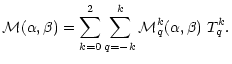
Equation (3) implies that the polarization matrix of the incident radiation can be written as the angular average ${\cal{J}}(\alpha,\beta,\nu)$ multiplied by a unitary matrix ${\cal{M}}(\alpha,\beta)$, which describes the angular behavior of the incident radiation coming in the direction ${\textbf{\textit{n}}}(\alpha,\beta)$ (for more details see Sahal-Bréchot  et al. 1998). The elements of the polarization matrix expanded on the irreducible tensor basis $\left\{T^k_q\right\}$ are obtained by expanding the matrix ${\cal{M}}(\alpha,\beta)$ in multipole terms on the same basis in the solar frame (Pxyz) ((Pz) is the quantization axis), thus

$${\cal M}(\alpha,\beta)=\sum_{k=0}^{2}\sum_{q=-k}^{k} {\cal M}^k_q(\alpha,\beta) \;T^k_q.$$ (4)

The matrix elements of $\varphi({\textbf{\textit{v}}}_{\scriptscriptstyle{\rm {A}}})$ developed on the irreducible tensor basis $\left\{T^k_q\right\}$, in the solar frame (Pxyz), are consequently given by

$$\begin{array}{ll} {\displaystyle \varphi^k_q({\textbf{\textit{v}}... ...) } \\ &{\displaystyle = {\cal{K}}\, {\cal M}^k_q(\alpha,\beta) .} \end{array}$$ (5)

For electric dipole transitions, we limit ourself to integer values of k between 0 and 2. k=0 gives the intensity component, k=1 gives the circular polarization components (which are zero if the incident radiation is unpolarized), and k=2 gives the linear polarization components. The computation of the matrix elements ${\cal M}^k_q(\alpha,\beta)$ is presented in Sahal-Bréchot et al. (1986). Their expressions are given also by Sahal-Bréchot et al. (1998).

The density matrix of an atom in interaction with its surrounding medium (incident photons and colliding particles) depends on the local magnetic field and eventually on the atomic velocity field. It is more practical to write the equations describing this interaction in the frame where the magnetic field vector is parallel to the quantization axis. This permits to keep the magnetic quantum number as a good quantum number. In addition, the density matrix elements of the reemitted photons are easily obtained in this frame. We note by $(PX^{\prime}Y^{\prime}Z^{\prime})$ the magnetic frame, the quantization axis $(PZ^{\prime})$ is parallel to the magnetic field vector. It is, so, necessary to rewrite the density matrix elements of the incident photons in the frame $(PX^{\prime}Y^{\prime}Z^{\prime})$ which is obtained from the solar one (Pxyz) by a rotation with the Euler angle $(\psi,\eta,0)$ ($\psi$ and $\eta$ are respectively the azimuth and the polar angle of the magnetic field vector in the frame (Pxyz)).

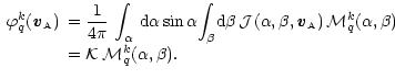
The formula giving the density matrix elements ${\phi^\prime}^k_q$ (relative to a frame ${\cal{R}^\prime}$) obtained from the elements ${\phi}^k_q$ (relative to a frame ${\cal{R}}$) through a rotation from ${\cal{R}}$ to ${\cal{R}^\prime}$ of angles $(\Omega, \Theta,\Psi)$ is given by (Bommier 1977)

$${\phi^\prime}^k_{q^\prime} = \sum^k_{q=-k} {\rm {e}}^{{\rm {i}}\;... ...^\prime\,\Psi \right)}\; {d}^k_{q^\prime q}\left(-\Theta\right)\; {\phi}^k_{q},$$ (6)

the coefficients ${d}^k_{q^\prime q}$ are given in Brink & Satchler (1962).

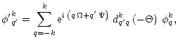
We note by $\varphi^\prime({\textbf{\textit{v}}}_{\scriptscriptstyle{\rm {A}}})$ the incident photons density matrix in $(PX^{\prime}Y^{\prime}Z^{\prime})$. The matrix elements of $\varphi^\prime({\textbf{\textit{v}}}_{\scriptscriptstyle{\rm {A}}})$ are obtained from those of $\varphi({\textbf{\textit{v}}}_{\scriptscriptstyle{\rm {A}}})$ by using the equation of the density matrix element transformation by an Euler rotation given by

$${\varphi^\prime}^k_{q^\prime}( {\textbf{\textit{v}}}_{\scriptscri... ... q}(-\eta) \; \varphi^k_q({\textbf{\textit{v}}}_{\scriptscriptstyle{\rm {A}}}).$$ (7)

The resulting matrix elements ${\varphi^\prime}^k_q({\textbf{\textit{v}}}_{\scriptscriptstyle{\rm {A}}})$ of the incident photons written in the magnetic field frame are given by

$$\begin{eqnarray*}\begin{array}{l} {\varphi^\prime}^0_0({\textbf{\textit{v}}}_{\s... ...f{\textit{v}}}_{\scriptscriptstyle{\rm {A}}})\right] \end{array}\end{eqnarray*}$$

$$\begin{array}{l} {\varphi^\prime}^2_1({\textbf{\textit{v}}}_{\scr... ...phi^2_2({\textbf{\textit{v}}}_{\scriptscriptstyle{\rm {A}}})\right] \end{array}$$ (8)

$$\begin{eqnarray*}\begin{array}{l} {\varphi^\prime}^2_2({\textbf{\textit{v}}}_{\s... ...f{\textit{v}}}_{\scriptscriptstyle{\rm {A}}})\right]. \end{array}\end{eqnarray*}$$

The symbols $\Re{\rm {e}}$ and $\Im{\rm {m}}$ design respectively the real and imaginary part of their arguments. To avoid the repetition of the previous expressions, we note

$${\varphi^\prime}^k_q({\textbf{\textit{v}}}_{\scriptscriptstyle{\rm {A}}}) ={\cal{K}}\,{\varphi^\prime}^k_q(\alpha,\beta,\eta,\psi)$$ (9)

${\varphi^\prime}^k_q(\alpha,\beta,\eta,\psi)$ is the angular term of the density matrix element ${\varphi^\prime}^k_q({\textbf{\textit{v}}}_{\scriptscriptstyle{\rm {A}}})$.

As mentioned in Sahal-Bréchot et al. (1998), the expressions obtained for the polarization matrix elements of the incident radiation are general and no restricting assumptions are made to this part. In order to get the density matrix of the reemitted photons which lead to the Stokes parameters of the scattered radiation, we should write and solve the statistical equilibrium equations describing the interaction of the moving atom with the incident radiation.