Designing an interferometric array consists mainly in choosing the locations of the stations (or pads) that will carry the antennas during the observations. In general more stations than antennas are planned to allow several configurations. An ideal design should ensure optimal configurations regarding all possible observation situations (source positions and durations of observation), scientific purposes (single field imaging, mosaicing, astrometry, detection, ...) and constraints (cost, ground composition and practicability, operation of the instrument, ...). The large number of parameters and sometimes incompatible specifications make this optimization problem complex and difficult to solve globally. The development of radio-interferometric instrumentation has given rise to several publications contributing to some aspects of the problem (e.g., Thompson et al. 1991; Cornwell 1986; Cornwell et al. 1993; Keto 1997; Conway 2000a,b; Kogan 1997; Woody 1999). This paper concentrates on the "configuration problem'' stated below which can be seen as a first step in the optimization process. A method able to solve this problem is proposed and guidelines on the way to use it for a full array design are presented.
The "configuration problem'' may be stated as follows: given,
This problem differs from the general "design problem'' since only a single observation situation and a single scientific purpose are considered. But, as will be shown below, getting over this first obstacle makes the full array design accessible. The relationship between the scientific purpose and the distribution of Fourier samples is central and deserves a complete analysis. This constitutes the subject of a second paper (Boone 2001b, hereafter Paper II).
An introduction and a very clear description of the configuration problem is given in Keto (1997). I shall only recall that for a zenithal snapshot observation the sampling function in Fourier plane (the function composed of Dirac ![]() -functions at the sample coordinates) is equal to the autocorrelation of the configuration function (the function composed of Dirac
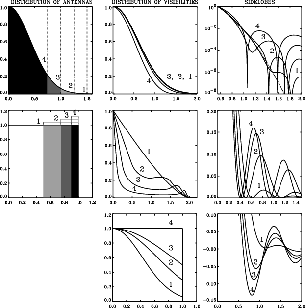
-functions at the sample coordinates) is equal to the autocorrelation of the configuration function (the function composed of Dirac ![]() -functions at the antenna coordinates) without the central point when the antennas are not correlated with themselves. Several examples are illustrated in Fig. 1 where the distribution of Fourier samples and the corresponding synthesized beam are given for some continuous two dimensional distributions of antennas. There is generally no distribution of antennas able to yield a distribution of samples equal to a given 2d-function, since this given function is not necessarily an autocorrelation. For example it can be shown that there is no solution for a uniform distribution: no 2d real positive function can yield a top hat function by autocorrelation. More generally an autocorrelation function is necessarily derivable and the distributions represented on the third row of Fig. 1 do not admit any solution for the distribution of antennas. But their properties, discussed in Paper II, are interesting and it might be worth deriving configurations yielding distributions as close as possible to those ones. Thus, "solving'' the configuration problem does not mean inverting an autocorrelation product but rather finding the configuration yielding the distribution of samples closest to the target one (it is an inverse problem). The use of an optimization method derives naturally from this observation.
-functions at the antenna coordinates) without the central point when the antennas are not correlated with themselves. Several examples are illustrated in Fig. 1 where the distribution of Fourier samples and the corresponding synthesized beam are given for some continuous two dimensional distributions of antennas. There is generally no distribution of antennas able to yield a distribution of samples equal to a given 2d-function, since this given function is not necessarily an autocorrelation. For example it can be shown that there is no solution for a uniform distribution: no 2d real positive function can yield a top hat function by autocorrelation. More generally an autocorrelation function is necessarily derivable and the distributions represented on the third row of Fig. 1 do not admit any solution for the distribution of antennas. But their properties, discussed in Paper II, are interesting and it might be worth deriving configurations yielding distributions as close as possible to those ones. Thus, "solving'' the configuration problem does not mean inverting an autocorrelation product but rather finding the configuration yielding the distribution of samples closest to the target one (it is an inverse problem). The use of an optimization method derives naturally from this observation.
This paper is organized as follows: in Sect. 2 the existing methods are briefly recalled and a new one based on pressure forces is introduced. Section 3 describes how the optimization convergence can be improved and the different kinds of observation (synthesis, multi-configuration, mosaicing) integrated in the implementation. In Sect. 4 the application of the method to various situations and guidelines for the full array design are presented. Section 5 gives the conclusion.
Copyright ESO 2001