 |
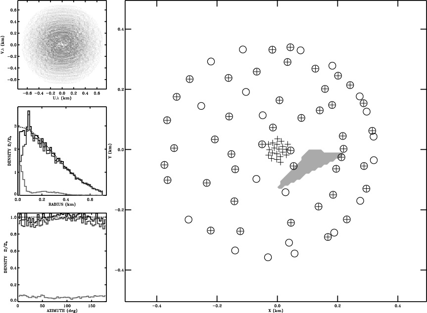
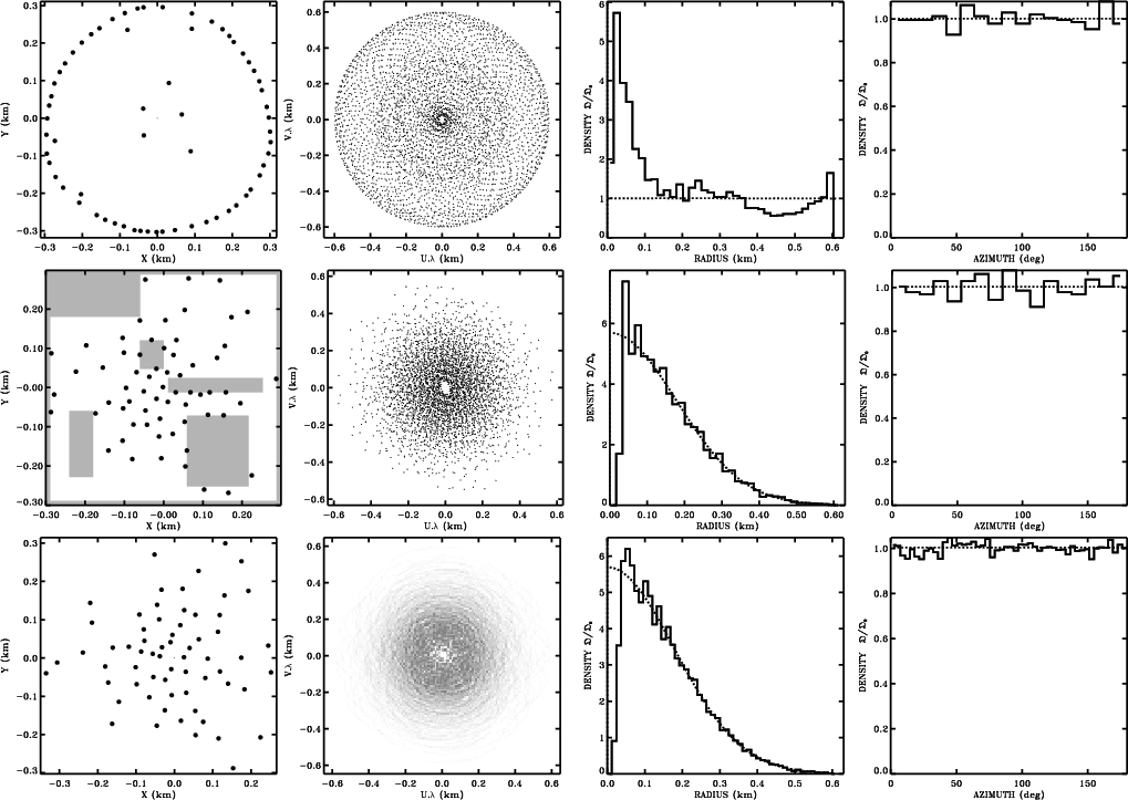
Figure 5: Examples of application. On the first row: optimization for a zenithal snapshot observation and a uniform model distribution of samples (dashed line in the profiles). Second row: same optimization as in Fig. 3 but with ground constraints: the forbidden regions are symbolized by the dark areas. Third row: optimization for the same Gaussian model distribution but for a 6 h-observation, 3 h on either side of the zenith. |
The execution speed and the convergence are highly dependent on the algorithm used for the computation of the density gradient. The simplest way to calculate this gradient is to count the number of Fourier samples in each cell of a grid, and then, the difference between adjacent cells. The choice of the grid is crucial for the convergence of the method. Consider the case of a Gaussian model distribution: if the grid is orthogonal many cells in the outer part of the distribution will be empty causing gradients with the neighbors which may contain only one sample. In other words the program will be sensible to gradients arising from the discrete nature of the sampling function. In addition it will give the same weight to a gradient over a region containing lots of samples in the center and a similar gradient concerning only a few samples on the outer part. Finally, the circular boundary will cross the square cells and the area of each of these cells being outside the boundary will depend upon the coordinates of the cell. The distribution at the boundaries will consequently be out of control.
For these reasons it is optimal to use an adaptive circular grid. That is, a circular grid for which the number of Fourier samples in each cell is constant when the distribution is equal to the model. Thus, in the Gaussian model example where the model density is given by:
 |
(4) |
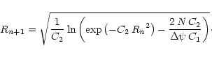 |
(5) |
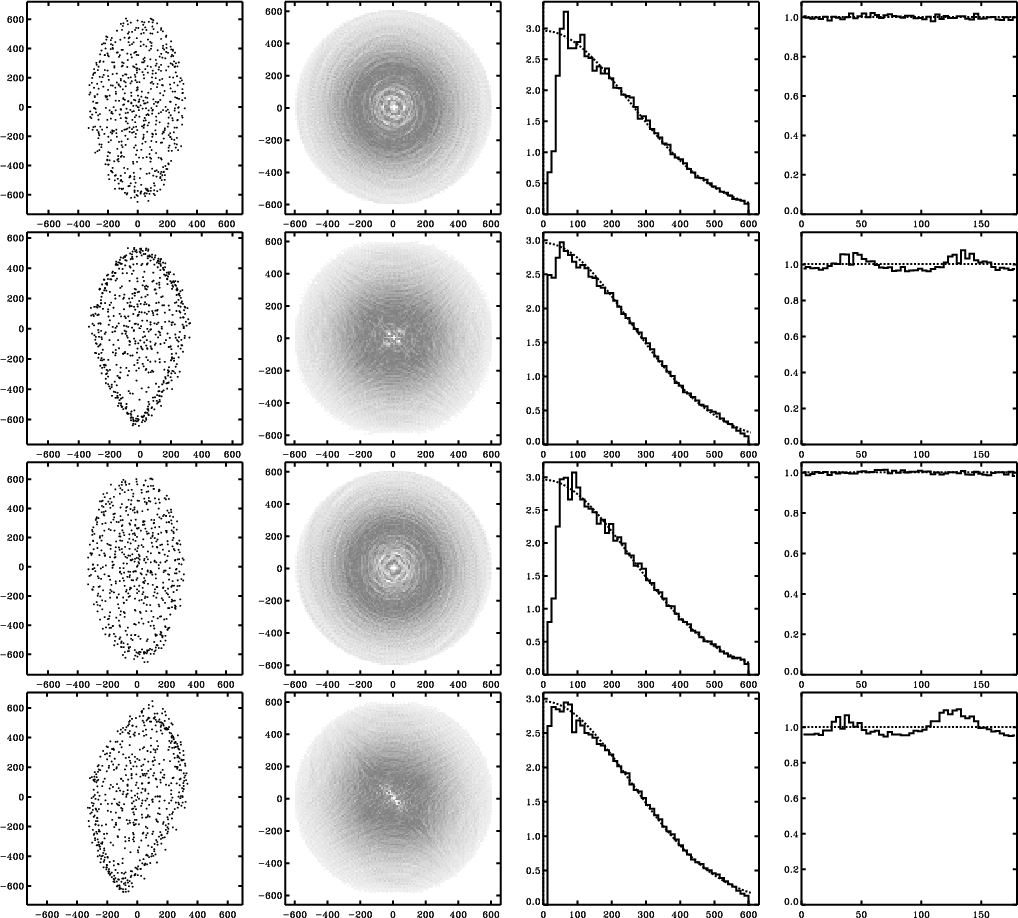
However, optimizing a configuration with only one grid do not ensure the resulting distribution of samples to fit the model at all resolutions. It can show strong defects at larger or smaller scales than the average cell size of the grid. In order to optimize the distribution at all resolutions simultaneously several grids have to be used simultaneously. For example to optimize a 64-antennas array it was found optimal to use 7 grids of sizes 62 up to 132 cells per quadrant.
For topography constraints the simplest situation has been considered: a digital mask was used to define forbidden regions for the antennas. When moving an antenna, if the destination falls into such a forbidden area the antenna is placed either before or after the area depending on which is the nearest to the original destination. More complex constraints may also be considered, e.g. in the form of pressure forces on the antennas arising from the local level of forbidding.
In the case of earth rotation synthesis the geometrical transformation from uv-plane to antenna plane, ![]() ,
is different for each sample of a given antenna pair, in addition different weights are given to the Fourier samples according to the elevation of the source, i.e. to the level of noise. The choice of the averaging time separating two measurements is a compromise between computing time and good sampling of the largest baseline track. It is not related to the real operation of the instrument. For example it can be taken equal to half an hour for a 8 h-observation: 16 points per track might be enough in the sense that taking more points would not change the resulting configuration.
,
is different for each sample of a given antenna pair, in addition different weights are given to the Fourier samples according to the elevation of the source, i.e. to the level of noise. The choice of the averaging time separating two measurements is a compromise between computing time and good sampling of the largest baseline track. It is not related to the real operation of the instrument. For example it can be taken equal to half an hour for a 8 h-observation: 16 points per track might be enough in the sense that taking more points would not change the resulting configuration.
Mosaicing (see e.g., Cornwell 1988; Cornwell et al. 1993) can be easily integrated in the program by allowing only segments of the tracks to be sampled. The unsampled parts correspond to the time spent on the other pointings of the mosaic. It is stressed however that the way the tracks are sampled, regularly or by segments in the case of mosaicing, has little impact on the configurations provided that the time spent on the other fields is not too long, i.e. the mosaic is not too large. As shown in Sect. 4 the curvature of the tracks described by the baselines has a strong impact as it determines the way they can be packed to make the density fit as well as possible the model distribution. This curvature is affected only when the separation between sampled segments is large i.e. greater than
![]() h. Hence, if 1 min is spent on each pointing, the mosaic has to be larger than 30 fields to have an impact on the configuration.
h. Hence, if 1 min is spent on each pointing, the mosaic has to be larger than 30 fields to have an impact on the configuration.
To handle multi-configuration observations the density is computed by adding the Fourier samples measured by all the configurations. Some antennas might take part in several configurations allowing for the situation in which only some of the antennas are moved before observing the same source again. For each configuration uv-plane constraints are given in the form of a maximum and minimum radius for the uv-ring to be sampled. The minimum radius constraint allows to exclude any shadowing between the antennas: shadowing happens when some Fourier samples are inside a radius equal to the projected antenna diameter.
A C++ library, named APO (Antenna Positions Optimization), was written to optimize the positions of the antennas of any instrument in any of those situations. The flexibility of the object oriented language is well adapted to the implementation of the method. Five main classes were defined corresponding to the description of an instrument, a site, an observational situation, a model distribution of samples and a grid. Each of these classes can be instantiated several times and the optimization can run on all objects. For instance it is possible to: create 7 different grids as mentioned above and run the optimization considering all of them; create several observational situations with an eventual weight for each of them and optimize the instrument accordingly; optimize several instruments on different sites in order to make them complementary regarding some observational situations and scientific purposes (i.e. distribution of samples).
Copyright ESO 2001