| q |
|
M50 |
|
| 0.3 | 6.7 | 3.90 | 197 |
| 0.5 | 7.2 | 4.02 | 201 |
| 0.8 | 8.1 | 4.21 | 208 |
| 1.0 | 8.7 | 4.32 | 212 |
The integrals in Eqs. (18) and (21) may be evaluated only numerically, but to do this we need to fix all the parameters entering the mass density in Eq. (12) (i.e. q,
![]() ,
R0,
,
R0, ![]() ), the lower and upper mass limits
), the lower and upper mass limits
![]() and also the slope
and also the slope ![]() of the MF which is just the parameter we want to determine.
of the MF which is just the parameter we want to determine.
We have fixed R0 = 8.0 kpc and
![]() kpc (as usual in literature). Next we have to choose the halo flattening q, but the constrains on it are really very poor. Different kinds of analysis with different techniques give very different results (for a review see, e.g., Rix 1996; Sackett 1999) and there is no general agreement on which value is the best one to use. Since there is such a large uncertainty, we have decided to consider four values of the halo flattening, repeating our analyses for models with
q = 0.3, 0.5, 0.8, 1.0 in order to test if this parameter has some effect on the results. The last parameter to fix is the local mass density for the spherical case
kpc (as usual in literature). Next we have to choose the halo flattening q, but the constrains on it are really very poor. Different kinds of analysis with different techniques give very different results (for a review see, e.g., Rix 1996; Sackett 1999) and there is no general agreement on which value is the best one to use. Since there is such a large uncertainty, we have decided to consider four values of the halo flattening, repeating our analyses for models with
q = 0.3, 0.5, 0.8, 1.0 in order to test if this parameter has some effect on the results. The last parameter to fix is the local mass density for the spherical case
![]() .
This is fixed such that the local rotation velocity is equal to the observed value of
.
This is fixed such that the local rotation velocity is equal to the observed value of
![]() km s-1. To this aim we have also considered the contributions of the bulge and disk. We modelled these components as in Méra
et al. (1998): the bulge is treated as point like with total mass
km s-1. To this aim we have also considered the contributions of the bulge and disk. We modelled these components as in Méra
et al. (1998): the bulge is treated as point like with total mass
![]() and the disk as a double exponential with scale length
and the disk as a double exponential with scale length
![]() kpc and local surface mass density
kpc and local surface mass density
![]() .
In Table 1 we give the values of the models parameters together with the total mass inside 50 kpc and the asymptotic rotation velocity. We would like to note that the predicted values of these latter quantities are in good agreement within the errors with the recent measurements (see, e.g., Wilkinson & Evans 1999) for all the considered models.
.
In Table 1 we give the values of the models parameters together with the total mass inside 50 kpc and the asymptotic rotation velocity. We would like to note that the predicted values of these latter quantities are in good agreement within the errors with the recent measurements (see, e.g., Wilkinson & Evans 1999) for all the considered models.
In order to obtain the observable in term of ![]() we have numerically integrated Eqs. (18) and (21) for many values of
we have numerically integrated Eqs. (18) and (21) for many values of ![]() and then interpolated the results to get
and then interpolated the results to get
![]() and
and ![]() as functions of
as functions of ![]() itself. We have then repeated this procedure changing the values for the halo flattening q and the mass limits in order to investigate a wide class of halo models, each one labelled with a code given as follows. We named A1, A2 models with
itself. We have then repeated this procedure changing the values for the halo flattening q and the mass limits in order to investigate a wide class of halo models, each one labelled with a code given as follows. We named A1, A2 models with
![]() and
and
![]() and
and
![]() respectively, and B1, B2 models with
respectively, and B1, B2 models with
![]() and
and
![]() and
and
![]() respectively. Then we add a letter to indicate the halo flattening with the following conventions:
respectively. Then we add a letter to indicate the halo flattening with the following conventions:
![]() ,
,
![]() ,
,
![]() ,
,
![]() .
So, e.g., the model labelled A2c has:
.
So, e.g., the model labelled A2c has:
![]() ,
,
![]() ,
q = 0.8. Thus, we consider sixteen different models in the same class.
,
q = 0.8. Thus, we consider sixteen different models in the same class.
Before going on, we would like to discuss how we have chosen the mass limits
![]() .
Concerning the upper limit, it has been known for a long time now (Gilmore & Hewett 1983) that hydrogen-burning stars cannot provide the majority of the halo dark matter. Numerous recent studies (Bahcall et al. 1994; Hu et al. 1994; Graff & Freese 1996) put an upper limit of at most 4% on the dark halo density contribution of hydrogen-burning stars. For an old, metal-poor population this means that stars with mass between 0.1
.
Concerning the upper limit, it has been known for a long time now (Gilmore & Hewett 1983) that hydrogen-burning stars cannot provide the majority of the halo dark matter. Numerous recent studies (Bahcall et al. 1994; Hu et al. 1994; Graff & Freese 1996) put an upper limit of at most 4% on the dark halo density contribution of hydrogen-burning stars. For an old, metal-poor population this means that stars with mass between 0.1![]() and 0.8
and 0.8![]() give no significant contribution to the dark matter in the galactic halo. These evidences suggest to fix
give no significant contribution to the dark matter in the galactic halo. These evidences suggest to fix
![]() ,
but we have decided to consider also models with
,
but we have decided to consider also models with
![]() for the reasons we are going to explain. On one hand, MACHO (Alcock et al. 2000a) and EROS (Renault et al. 1997) results indicate that the most likely MACHO' s mass is
for the reasons we are going to explain. On one hand, MACHO (Alcock et al. 2000a) and EROS (Renault et al. 1997) results indicate that the most likely MACHO' s mass is
![]() .
On the other hand, Kerins (1997) has shown that MACHOs may reside in a population of dim halo globular clusters comprising mostly or entirely low-mass stars just above the hydrogen-burning limit. For the case of the standard halo model, this scenario is consistent not only with MACHO observations, but also with cluster dynamical constraints and number counts limits imposed by twenty HST fields. Further suggestions of the possible existence of MACHOs with mass
.
On the other hand, Kerins (1997) has shown that MACHOs may reside in a population of dim halo globular clusters comprising mostly or entirely low-mass stars just above the hydrogen-burning limit. For the case of the standard halo model, this scenario is consistent not only with MACHO observations, but also with cluster dynamical constraints and number counts limits imposed by twenty HST fields. Further suggestions of the possible existence of MACHOs with mass
![]() come from the study of the double quasars variability (Koopmans & de Bruyn 2000). All these studies have led us to consider also models with
come from the study of the double quasars variability (Koopmans & de Bruyn 2000). All these studies have led us to consider also models with
![]() .
.
| q |
|
|
|
|
||||
| 0.3 | 0.08 | 0.22 | -8.83 | 3.42 | 0.13 | -0.09 | -8.67 | 7.00 |
| 0.5 | 0.08 | 0.23 | -8.84 | 3.94 | 0.13 | -0.09 | -8.67 | 7.57 |
| 0.8 | 0.08 | 0.24 | -8.84 | 4.26 | 0.13 | -0.09 | -8.67 | 7.92 |
| 1.0 | 0.08 | 0.24 | -8.84 | 4.36 | 0.13 | -0.09 | -8.67 | 8.02 |
| 0.3 | 0.17 | 0.35 | -11.33 | 7.48 | 0.29 | -0.47 | -10.67 | 11.92 |
| 0.5 | 0.17 | 0.38 | -11.35 | 7.98 | 0.29 | -0.47 | -10.67 | 12.47 |
| 0.8 | 0.17 | 0.39 | -11.36 | 8.29 | 0.29 | -0.46 | -10.68 | 12.81 |
| 1.0 | 0.16 | 0.40 | -11.37 | 8.38 | 0.29 | -0.46 | -10.68 | 12.91 |
| q |
|
|
|
|
||||
| 0.3 | 0.008 | 0.16 | -8.75 | 3.38 | 0.02 | 0.10 | -8.81 | 7.02 |
| 0.5 | 0.008 | 0.16 | -8.75 | 3.89 | 0.02 | 0.10 | -8.81 | 7.58 |
| 0.8 | 0.009 | 0.16 | -8.74 | 4.21 | 0.02 | 0.10 | -8.81 | 7.93 |
| 1.0 | 0.008 | 0.16 | -8.75 | 4.31 | 0.02 | 0.10 | -8.81 | 8.04 |
| 0.3 | 0.05 | 0.42 | -11.23 | 7.44 | 0.12 | -0.01 | -11.02 | 11.98 |
| 0.5 | 0.05 | 0.43 | -11.23 | 7.93 | 0.12 | 0.004 | -11.02 | 12.53 |
| 0.8 | 0.05 | 0.43 | -11.24 | 8.24 | 0.12 | 0.007 | -11.02 | 12.87 |
| 1.0 | 0.05 | 0.43 | -11.24 | 8.34 | 0.12 | 0.008 | -11.02 | 12.97 |
Fixing the lower limit
![]() is not an easy task too. De Rujula et al. (1991) have shown that a lower limit for the mass of MACHOs is
is not an easy task too. De Rujula et al. (1991) have shown that a lower limit for the mass of MACHOs is
![]() ,
but this does not imply that objects with a mass
,
but this does not imply that objects with a mass
![]() really exist. Actually, MACHO and EROS search for short duration events pose strong constraints on their contribution to the halo mass budget (Alcock et al. 1996; Alcock et al. 1998; Renault et al. 1998). Following these works, we have chosen two values for
really exist. Actually, MACHO and EROS search for short duration events pose strong constraints on their contribution to the halo mass budget (Alcock et al. 1996; Alcock et al. 1998; Renault et al. 1998). Following these works, we have chosen two values for
![]() given by 0.001 and 0.01 respectively. In all our analysis we are assuming that the MF is the same in the mass range
given by 0.001 and 0.01 respectively. In all our analysis we are assuming that the MF is the same in the mass range
![]() ,
i.e. that the slope
,
i.e. that the slope ![]() does not change in this range, which seems quite reasonable as a first approximation.
does not change in this range, which seems quite reasonable as a first approximation.
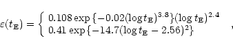
To integrate Eqs. (18) and (21) we need the detection efficiency of the MACHO collaboration for their monitoring campaign towards LMC since in our analysis we will use their results of the first 5.7 years of observations. This function has been carefully evaluated by the MACHO group itself (Alcock et al. 2000b), but they give no analytical formula for it. That is why we have built up an approximated expression of
![]() interpolating the data taken from Fig. 5 of Alcock et al. (2000a), obtaining
interpolating the data taken from Fig. 5 of Alcock et al. (2000a), obtaining
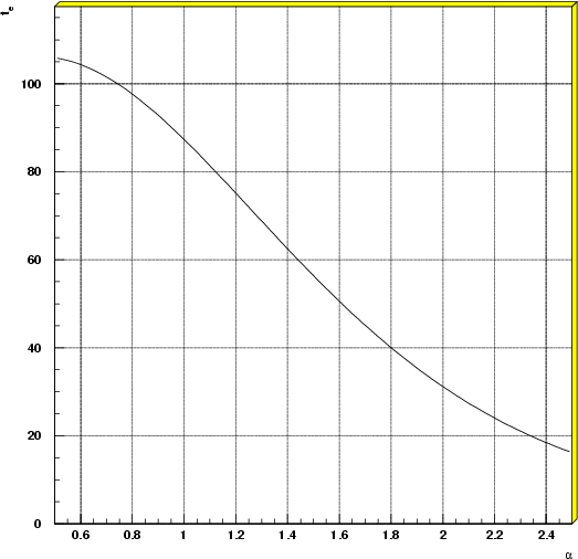 |
Figure 1:
|
Now we have all we need to estimate the functions defined in Eqs. (18) and (21). Without entering in details, the numerical integration and the following interpolation of the results have shown us that it is possible to write
Copyright ESO 2001