Internal errors on the astrometry may also be discussed from a consistency check between the
observation sequences made in several filters. We verified the assumption that relative positions are independent from the filter choice by computing the "distance'' d, i.e.
the difference in relative positions for the filters V and i, as
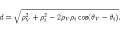 |
(2) |
Some programme and astrometric standard stars were observed twice or more (see Table 3).
As mentioned before, these regularly observed double stars are important to check the consistency between observations obtained at different epochs. There is indeed an excellent agreement between the measurements of the same star as can be deduced from the small standard deviations both in angular separation and in position angle. For example, we can check the wide astrometric pairs with observations obtained at different epochs: BD +13
![]() 3203 (+1303203a, n=5), BD -22
3203 (+1303203a, n=5), BD -22
![]() 1505 (32144a, n=4), BD -56
1505 (32144a, n=4), BD -56
![]() 256 (5843a, n=7) in Table 3. Their
standard deviations fluctuate between 0.003 to 0.005
256 (5843a, n=7) in Table 3. Their
standard deviations fluctuate between 0.003 to 0.005
![]() in angular separation and between 0.01 to 0.02
in angular separation and between 0.01 to 0.02![]() in positional angle.
in positional angle.
![\begin{figure}
\par\includegraphics[angle=270,width=8.8cm,clip]{H2285.fig3.eps}
\end{figure}](/articles/aa/full/2001/28/aah2285/img72.gif) |
Figure 3:
Differences in angular separation between filters
V and i. Unfilled diamonds represent the 15 systems with |
![\begin{figure}
\par\includegraphics[angle=270,width=8.8cm,clip]{H2285.fig4.eps}
\end{figure}](/articles/aa/full/2001/28/aah2285/img73.gif) |
Figure 4:
Internal errors on mean differential V magnitude vs. angular separation for two classes of |
We discuss here both internal errors: those on the differential photometry only and those
of the absolute photometry (obtained through calibration of standard stars). In the former case,
the internal photometric errors depend on the repeatability of the differences of the
component magnitudes. The internal consistency of
these differences can be assessed by inspection of the standard deviations listed in Table 3.
Figure 4 represents the distribution of the internal errors on the differential V magnitude plotted as a function of angular separation for two different ranges of ![]() .
The mean internal error is well below 0.01 mag but there is evident degradation at
larger differential magnitudes. In the worst case of a combination of a small separation
(
.
The mean internal error is well below 0.01 mag but there is evident degradation at
larger differential magnitudes. In the worst case of a combination of a small separation
(![]() < 3
< 3
![]() )
and a large difference of magnitude (
)
and a large difference of magnitude (
![]() mag), this error tends to increase to a few tenths of a magnitude. A similar figure applies to the differential I magnitudes.
The multiply observed astrometric standard stars BD +13
mag), this error tends to increase to a few tenths of a magnitude. A similar figure applies to the differential I magnitudes.
The multiply observed astrometric standard stars BD +13
![]() 3203 (n=5),
BD -22
3203 (n=5),
BD -22
![]() 1505 (n=4) and BD -56
1505 (n=4) and BD -56
![]() 256 (n=7) from Table 3
show the same tendency: we find millimag consistency on the differential magnitudes in the case
of BD +13
256 (n=7) from Table 3
show the same tendency: we find millimag consistency on the differential magnitudes in the case
of BD +13
![]() 3203 (
3203 (
![]() ), some hundreths of a magnitude for
), some hundreths of a magnitude for
![]() and more than 0.1 mag in the case of BD -56
and more than 0.1 mag in the case of BD -56
![]() 256 (
256 (
![]() )
shown hereafter to be variable.
In the latter case - under favourable photometric conditions - several standard stars have been observed to which classical colour equations have been applied. We have taken into consideration
a transformation error (generally 0.02-0.03 mag) depending on the quality of each night
as well as an error (usually insignificant) on the joint magnitude of the system to compute the
individual errors on the component magnitudes which are also listed in Table 4
(Paper I, Sect. 4.3).
The mean errors on the magnitudes and the indices (V-I) of the components A and B deduced from Table 4 respectively give the following values:
)
shown hereafter to be variable.
In the latter case - under favourable photometric conditions - several standard stars have been observed to which classical colour equations have been applied. We have taken into consideration
a transformation error (generally 0.02-0.03 mag) depending on the quality of each night
as well as an error (usually insignificant) on the joint magnitude of the system to compute the
individual errors on the component magnitudes which are also listed in Table 4
(Paper I, Sect. 4.3).
The mean errors on the magnitudes and the indices (V-I) of the components A and B deduced from Table 4 respectively give the following values:
![]() ,
,
![]() ,
,
![]() and
and
![]() mag. For the sample of binaries with
mag. For the sample of binaries with ![]() < 3
< 3
![]() and
and
![]() ,
these values rise to
,
these values rise to
![]() ,
,
![]() ,
,
![]() and
and
![]() mag.
mag.
| Identifier | Jul. Dat. | nI |
|
|
|||
| 2440000+ | (mag) | (mag) | (mag) | (mag) | (mag) | ||
| 005843a | 9348.4085 | 3 | 5.904 | .017 | 11.173 | .061 | 5.269 |
| 079902 | 8851.5582 | 16 | 7.816 | .020 | 10.801 | .020 | 2.985 |
| 088603 | 8850.6143 | 13 | 8.658 | .020 | 10.720 | .020 | 2.062 |
| 109156 | 8850.7526 | 4 | 9.102 | .020 | 12.706 | .020 | 3.604 |
| 117316 | 8850.8339 | 11 | 9.647 | .020 | 12.601 | .020 | 2.954 |
| Identifier | Jul. Dat. | nV |
|
|
nI |
|
|
|
|
Code | ||||
| 011219 | 9668.7130 | 10 | 8.864 | 0.020 | 10.129 | 0.020 | 0 | - | - | - | - | 1.265 | - | LO |
| 011219 | 8549.7389 | 4 | 8.842 | 0.016 | 10.132 | 0.016 | 4 | 0.969 | 0.017 | 0.630 | 0.021 | 1.290 | -0.340 | CS |
| 022463 | 8941.7542 | 3 | 8.958 | 0.015 | 9.763 | 0.016 | 2 | 0.51 | 0.02 | 0.64 | 0.02 | .805 | 0.13 | LO |
| 022463 | 8550.7998 | 6 | 8.960 | 0.014 | 9.770 | 0.014 | 3 | 0.539 | 0.017 | 0.661 | 0.017 | 0.810 | 0.122 | CS |
| 042581a | 9345.6621 | 3 | 7.738 | 0.020 | 9.910 | 0.025 | 0 | - | - | - | - | 2.172 | - | LO |
| 042581a | 8671.6577 | 6 | 7.712 | 0.016 | 9.933 | 0.024 | 3 | 0.734 | 0.018 | 0.734 | 0.027 | 2.221 | 0.000 | CS |
| 114378a | 8850.7841 | 3 | 6.543 | 0.020 | 10.275 | 0.021 | 1 | 0.60 | 0.03 | 1.56 | 0.03 | 3.731 | 0.97 | LO |
| 114378a | 8548.6123 | 16 | 6.572 | 0.011 | 10.276 | 0.020 | 13 | 0.594 | 0.019 | 1.564 | 0.017 | 3.704 | 0.970 | CS |
External photometric errors can be evaluated from observations of the same target
acquired during different nights or different campaigns. For this we consider
the multiple observations of some astrometric standard stars (BD +13
![]() 3203 (+1303203a, n=5), BD -22
3203 (+1303203a, n=5), BD -22
![]() 1505 (32144a, n=2), BD -45
1505 (32144a, n=2), BD -45
![]() 13443 (97593a, n=2))
as well as some programme stars (HIP 2438, HIP 20020) listed in Table 4.
In addition, we also consider the objects in common with Paper II
(see Table 6). The case of BD -56
13443 (97593a, n=2))
as well as some programme stars (HIP 2438, HIP 20020) listed in Table 4.
In addition, we also consider the objects in common with Paper II
(see Table 6). The case of BD -56
![]() 256 (5843a, n=5)
is not included since we note significant variations between individual measurements as
well as a difference of 0.1 mag between our measurements and those reported in Paper II.
This confirms the variability detected by Hipparcos for this red giant of spectral type M2/3III.
Taking into consideration the nine objects previously cited, we find
256 (5843a, n=5)
is not included since we note significant variations between individual measurements as
well as a difference of 0.1 mag between our measurements and those reported in Paper II.
This confirms the variability detected by Hipparcos for this red giant of spectral type M2/3III.
Taking into consideration the nine objects previously cited, we find
![]() and
and
![]() mag. If we remove only one star (HIP 20020) we obtain
mag. If we remove only one star (HIP 20020) we obtain
![]() and
and
![]() mag. We thus are confident that the errors quoted in Table 4 are very realistic upper limits.
mag. We thus are confident that the errors quoted in Table 4 are very realistic upper limits.
![\begin{figure}
\par\includegraphics[height=6.0cm,angle=270,width=8.8cm,clip]{H2285.fig5.eps}
\end{figure}](/articles/aa/full/2001/28/aah2285/img96.gif) |
Figure 5: Difference between V component magnitudes in the sense CCD minus photoelectric versus angular separation. |
![\begin{figure}
\par\includegraphics[height=6.0cm,angle=270,width=8.8cm,clip]{H2285.fig6.eps}
\end{figure}](/articles/aa/full/2001/28/aah2285/img97.gif) |
Figure 6: Difference between V component magnitudes in the sense CCD minus photoelectric versus differential magnitude. |
![\begin{figure}
\par\includegraphics[angle=270,width=8.8cm,clip]{H2285.fig7.eps}
\end{figure}](/articles/aa/full/2001/28/aah2285/img98.gif) |
Figure 7:
Difference between total
|
![\begin{figure}
\includegraphics[angle=270,width=8.8cm,clip]{H2285.fig8.eps}
\end{figure}](/articles/aa/full/2001/28/aah2285/img99.gif) |
Figure 8:
Histogram of differences between total
|
We searched existing data bases for component photoelectric photometry. We have systematically
searched in the UBV, Strömgren and Geneva photometries since these systems have
the highest probability of success. Apart from the component photometry of the Double and
Multiple Systems Annex (vol. 10 of the Hipparcos Catalogue, ESA 1997), we found individual information
for 11 primary and 5 secondary components of our sample only making use mostly of the Lausanne
Photometric data base (Mermilliod et al. 1996) and for some systems of the Besançon Double and Multiple Star data base (Kundera et al. 1999). In Figs. 5
and 6 we illustrate the comparison as a function of angular separation and
magnitude difference: HIP 3397 (
![]() 14
14
![]() and colours of a giant) has a small deviation for the primary but a large
difference (>0.1 mag) for the secondary component; the primary component of
HIP 9258 (
and colours of a giant) has a small deviation for the primary but a large
difference (>0.1 mag) for the secondary component; the primary component of
HIP 9258 (
![]() 9
9
![]() )
turned out to be a variable star (a discordant previous measurement had mistakenly been attributed to the B companion)
so the deviation of 0.05 mag is not surprising. Except for
HIP 113386 (
)
turned out to be a variable star (a discordant previous measurement had mistakenly been attributed to the B companion)
so the deviation of 0.05 mag is not surprising. Except for
HIP 113386 (
![]() 9
9
![]() )
where both Strömgren and Geneva values are off by as much as
0.08 mag (no reason
found); the same effect is also seen on the difference between the joint V Johnson and CCD magnitude), the agreement is excellent for the primaries, with a mean deviation of +0.006 mag and a scatter of 0.022 mag only. In general the agreement is really good for the primary star but worse on the
secondary component. The published mean error is of the same order as the scatter found in
the differences between the CCD and the photoelectrically measured component magnitudes
(
)
where both Strömgren and Geneva values are off by as much as
0.08 mag (no reason
found); the same effect is also seen on the difference between the joint V Johnson and CCD magnitude), the agreement is excellent for the primaries, with a mean deviation of +0.006 mag and a scatter of 0.022 mag only. In general the agreement is really good for the primary star but worse on the
secondary component. The published mean error is of the same order as the scatter found in
the differences between the CCD and the photoelectrically measured component magnitudes
(![]() 0.02 mag). Even though the data are few, there is a possible trend when
one considers both figures together: the discrepancies are more frequent at large separations
and large differences of magnitude.
0.02 mag). Even though the data are few, there is a possible trend when
one considers both figures together: the discrepancies are more frequent at large separations
and large differences of magnitude.
More comparison data are available for the combined photometry of these systems: 122
double
stars have either UBV or Strömgren or Geneva combined photometry. We have 62 common pairs with Johnson, 70 with Strömgren and 64 with Geneva photometry. Total CCD
magnitudes have been recomputed from standard component magnitudes. A histogram of the
differences is shown in Fig. 10 where the gray zone refers to the differences
with the Strömgren photoelectric photometry. After removal of the "outlier'' cases at
the 3-![]() level for which the differences are larger than 0.1 mag in absolute value (including 10 different objects), the mean deviations and scatters are:
level for which the differences are larger than 0.1 mag in absolute value (including 10 different objects), the mean deviations and scatters are:
![\begin{figure}
\par\includegraphics[angle=270,width=8.8cm,clip]{H2285.fig9.eps}
\par\end{figure}](/articles/aa/full/2001/28/aah2285/img106.gif) |
Figure 9:
Same data as in Fig. 7: difference between total
|
Copyright ESO 2001
![\begin{figure}
\par\includegraphics[angle=270,width=8.8cm,clip]{H2285.fig10.eps}
\end{figure}](/articles/aa/full/2001/28/aah2285/img107.gif)