forest
 (
(
 )
)

forest
For a given column density range, combined
HST and ground-based observations have provided
evidence for
a change in the line number density evolution at
 :
a rapid evolution at z > 1.7 and
a slow evolution at z < 1.7 (Impey et al. 1996;
Riediger et al. 1998;
Weymann et al. 1998; Davé et al. 1999).
These observations have led to a speculation of
two distinct populations in the Ly
forest: a rapidly
evolving population which dominates at higher z and
a slowly evolving population which dominates at lower z.
:
a rapid evolution at z > 1.7 and
a slow evolution at z < 1.7 (Impey et al. 1996;
Riediger et al. 1998;
Weymann et al. 1998; Davé et al. 1999).
These observations have led to a speculation of
two distinct populations in the Ly
forest: a rapidly
evolving population which dominates at higher z and
a slowly evolving population which dominates at lower z.
Our results at
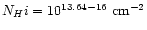 suggest that the transition from
the stronger evolution to the weaker evolution in
dn/dz occurs at
suggest that the transition from
the stronger evolution to the weaker evolution in
dn/dz occurs at
 (UM18
fits in the picture and is not an outlier), rather than
at
as suggested by previous observations and numerical simulations.
To be conservative, our
results show that dn/dz
at
continues to decrease at
a similar rate from
(UM18
fits in the picture and is not an outlier), rather than
at
as suggested by previous observations and numerical simulations.
To be conservative, our
results show that dn/dz
at
continues to decrease at
a similar rate from
 ,
with
a suggestion of slowing down in the evolution towards lower z.
,
with
a suggestion of slowing down in the evolution towards lower z.
The physics of the Ly
forest at z > 2 is
determined mainly by the Hubble expansion and the ionizing background,
 (or the H I photoionization rate,
 ).
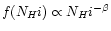
If the forest is "fixed" in comoving coordinates
for q0 = 0.5 and
).
If the forest is "fixed" in comoving coordinates
for q0 = 0.5 and
 ,
the observed number density of the Ly
forest is
proportional to
,
the observed number density of the Ly
forest is
proportional to
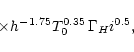
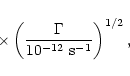
![$[(1+z)^{5} \, \Gamma_H{\sc i}^{-1}(z)]^{\beta-1}
\, (1+z)^{-3/2}$](/articles/aa/full/2001/27/aah2407/img432.gif) ,
where
,
where  is from
 .
This implies that dn/dz for a given column density
threshold decreases as z decreases
(Miralda-Escudé et al. 1996; Davé et al. 1999).
If we assume
.
This implies that dn/dz for a given column density
threshold decreases as z decreases
(Miralda-Escudé et al. 1996; Davé et al. 1999).
If we assume
 ,
dn/d
,
dn/d
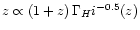 .
For a constant
,
this is much lower than
the observed index of dn/dz,
.
For a constant
,
this is much lower than
the observed index of dn/dz,
 ,
suggesting structure evolution and/or
evolution in dn/dz.
,
suggesting structure evolution and/or
evolution in dn/dz.
Recent numerical simulations
suggest that a decrease of
at z < 2plays a more important role to change the slope in
dn/dz at
due to the decreasing
QSO luminosity function at
z < 2 (Davé et al. 1999;
Riediger et al. 1998; Theuns et al. 1998;
Zhang et al. 1998).
The discrepancy between our observations and simulations
could be due to limited box sizes at z < 2 in
most simulations (losing large-scale power),
to numerical resolutions (underestimating
 or the number of lines at lower z) or to incorrect
.
If we take the results from most simulations
that
is the main drive of the
slope change in dn/dz, this discrepancy could simply indicate that
or the number of lines at lower z) or to incorrect
.
If we take the results from most simulations
that
is the main drive of the
slope change in dn/dz, this discrepancy could simply indicate that
 in most simulations,
i.e. the QSO-dominated Haardt-Madau
(Haardt & Madau 1996),
is underestimated at z < 2 and
that
at z < 2changes more slowly than a QSO-dominated
,
i.e.
there is a non-negligible contribution from galaxies at z < 2.
in most simulations,
i.e. the QSO-dominated Haardt-Madau
(Haardt & Madau 1996),
is underestimated at z < 2 and
that
at z < 2changes more slowly than a QSO-dominated
,
i.e.
there is a non-negligible contribution from galaxies at z < 2.
(
)
Assuming a truncated Gaussian b distribution with a lower
 -independent
 ,
Kim et al. (1997) concluded that over
,
Kim et al. (1997) concluded that over
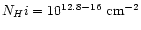 increases as z decreases: 15 km s-1 at
 ,
17 km s-1at
,
17 km s-1at
 ,
20 km s-1 at
,
20 km s-1 at
 ,
and 22-24 km s-1at
,
and 22-24 km s-1at
 .
This result has been explained by an additional heating
due to the on-going
He II reionization, although the high
value at
does not agree with any theoretical explanations (Kim et al. 1997;
Haehnelt & Steinmetz 1998;
Theuns et al. 2000b; Schaye et al. 2000).
.
This result has been explained by an additional heating
due to the on-going
He II reionization, although the high
value at
does not agree with any theoretical explanations (Kim et al. 1997;
Haehnelt & Steinmetz 1998;
Theuns et al. 2000b; Schaye et al. 2000).
Subsequent studies on
the z-evolution of
have led to contradictory results.
While
is clearly dependent
on
(Kirkman & Tytler 1997; Zhang et al. 1997),
 and the mean b value at
 (Kirkman & Tytler 1997) and at
 (Savaglio et al. 1999)
does not show any noticeable difference compared with at z > 3.
Combining the observations with the numerical simulations,
Schaye et al. (2000) found
that
at the fixed overdensity
(Savaglio et al. 1999)
does not show any noticeable difference compared with at z > 3.
Combining the observations with the numerical simulations,
Schaye et al. (2000) found
that
at the fixed overdensity  ,
,
 ,
increases from
,
increases from
 (
(
 kms-1) to
  (
(
 kms-1)
due to He II reionization at and then decreases from
(
kms-1) to
kms-1)
due to He II reionization at and then decreases from
(
kms-1) to
 (
(
 kms-1).
Ricotti et al. (2000) also found a similar increase in
at ,
although their
at z > 2.8 and at z < 2.8 can be considered to be constant
at
kms-1 and at
kms-1).
Ricotti et al. (2000) also found a similar increase in
at ,
although their
at z > 2.8 and at z < 2.8 can be considered to be constant
at
kms-1 and at
 km s-1, respectively.
On the other hand, adopting a slightly different approach for
identifying absorption lines instead of the Voigt profile fitting,
McDonald et al. (2000) found that there is
no
evolution over
2.1 < z < 4.4 at
the slightly higher overdensity
km s-1, respectively.
On the other hand, adopting a slightly different approach for
identifying absorption lines instead of the Voigt profile fitting,
McDonald et al. (2000) found that there is
no
evolution over
2.1 < z < 4.4 at
the slightly higher overdensity
 .
.
Figure 21 shows
the cutoff b values at the fixed column density
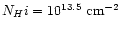 ,
,
 ,
from the two
power law fits in Sect. 4.3 as a function of z.
Keep in mind that
from the iterative power law fit is an upper limit, while
from the smoothed b distribution
is a lower limit.
The
value
shows a slight increase with decreasing zfrom both power law fits, with a possible local
maximum at
(with the caveat that the line list of
Q0302-003 is generated by a different fitting program
with respect to the other line lists. This could introduce an
artificial result at
as shown in Sect. 5.4, although
its redshift range suggests an influence of additional heating
if He II reionization does occur at ).
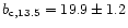
When all the values from both
fits are averaged,
,
from the two
power law fits in Sect. 4.3 as a function of z.
Keep in mind that
from the iterative power law fit is an upper limit, while
from the smoothed b distribution
is a lower limit.
The
value
shows a slight increase with decreasing zfrom both power law fits, with a possible local
maximum at
(with the caveat that the line list of
Q0302-003 is generated by a different fitting program
with respect to the other line lists. This could introduce an
artificial result at
as shown in Sect. 5.4, although
its redshift range suggests an influence of additional heating
if He II reionization does occur at ).
When all the values from both
fits are averaged,
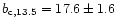 at
at
 is
smaller than
is
smaller than
 at
at
 ,
but the difference is significant only at the
,
but the difference is significant only at the
 level.
In simulations,
is usually measured at a fixed
overdensity  rather than at a fixed column density. Translating
an overdensity into the corresponding column density is not
trivial and depends on many uncertain parameters, such as
the ionizing background and the reionization history.
If the simple law between
and
by Davé
et al. (1999)
rather than at a fixed column density. Translating
an overdensity into the corresponding column density is not
trivial and depends on many uncertain parameters, such as
the ionizing background and the reionization history.
If the simple law between
and
by Davé
et al. (1999)![[*]](/icons/foot_motif.gif) is assumed,
then
becomes:
is assumed,
then
becomes:
,
the corresponding
is
 ,
,
 ,
,
 ,
,
 ,
,
 and
and
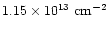 at
at
 3.75, 2.87, 2.66, 2.13, 1.98 and 1.61,
respectively. Although this conversion does not include
the effects of the He II reionization,
we assume that it is correct at least
on a relative scale at
and at
,
where the He II reionization
would not affect the temperature of the IGM as strongly as
at .
Therefore, we only discuss the relative behavior of
as a function of z, in particular,
our
at
with other results mentioned above.
3.75, 2.87, 2.66, 2.13, 1.98 and 1.61,
respectively. Although this conversion does not include
the effects of the He II reionization,
we assume that it is correct at least
on a relative scale at
and at
,
where the He II reionization
would not affect the temperature of the IGM as strongly as
at .
Therefore, we only discuss the relative behavior of
as a function of z, in particular,
our
at
with other results mentioned above.
For the iterative power law fit (the power law fit to the
smoothed b distribution), the b value at ,
,
is 20.8 (17.2),
20.1 (17.2), 19.4 (17.8), 20.5 (17.5), 22.4 (21.6)
and 20.4 (18.8) km s-1 at
3.75, 2.87, 2.66, 2.13, 1.98 and 1.61, respectively.
In the second panel of Fig. 21,
is fairly
constant with z as
 17-20 km s-1,
with a
possible local maximum
22 km s-1at
.
The observed behavior of
is qualitatively
in agreement with the results from McDonald et al. (2000).
While the observations agree with the fairly constant
at z < 3 derived by Ricotti et al. (2000),
they do not show the abrupt increase of
across
as large as
17-20 km s-1,
with a
possible local maximum
22 km s-1at
.
The observed behavior of
is qualitatively
in agreement with the results from McDonald et al. (2000).
While the observations agree with the fairly constant
at z < 3 derived by Ricotti et al. (2000),
they do not show the abrupt increase of
across
as large as
 7 km s-1 found by Ricotti et al.
The observations at
and at
agree with the results by Schaye et al. (2000)
which show similar
at
and at
.
In addition,
the observations do not show
a strong decrease of
from
to
7 km s-1 found by Ricotti et al.
The observations at
and at
agree with the results by Schaye et al. (2000)
which show similar
at
and at
.
In addition,
the observations do not show
a strong decrease of
from
to  as large as 4 km s-1 as found by Schaye et al. (2000).
However, note that, considering the large error bars of Schaye et al.
(2000), the significance of the decrease of
from
to
is not very strong and their
result is not in disagreement with ours.
It should also be recalled that we are
using the scaling law between
and
estimated from the QSO-dominated
Haardt-Madau
.
If this
QSO-dominated UV background is underestimated at z < 2as suggested by the evolution of the absorption line number density,
the actual
at z < 2.4 can be higher than
in Fig. 21.
as large as 4 km s-1 as found by Schaye et al. (2000).
However, note that, considering the large error bars of Schaye et al.
(2000), the significance of the decrease of
from
to
is not very strong and their
result is not in disagreement with ours.
It should also be recalled that we are
using the scaling law between
and
estimated from the QSO-dominated
Haardt-Madau
.
If this
QSO-dominated UV background is underestimated at z < 2as suggested by the evolution of the absorption line number density,
the actual
at z < 2.4 can be higher than
in Fig. 21.
The third panel of Fig. 21 shows the median
b values as a function of z measured for two column density ranges:
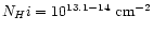 and
and
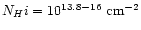 .
It is rather difficult to interpret
the z-dependence of the median bvalues. It could be constant at
1.5 < z < 4 with a small cosmic
variance at .
On the other hand, it could be decreasing
with z at z < 3.1, if we discard the median b values at
.
It is rather difficult to interpret
the z-dependence of the median bvalues. It could be constant at
1.5 < z < 4 with a small cosmic
variance at .
On the other hand, it could be decreasing
with z at z < 3.1, if we discard the median b values at
 ,
based on a small number of absorption lines.
Although simulations correctly predict the shape
of the observed b distributions,
the predicted median b values are typically 5-10 km s-1smaller than the observed ones at all z(Bryan & Machacek 2000; Machacek et al. 2000;
Theuns et al. 2000b).
,
based on a small number of absorption lines.
Although simulations correctly predict the shape
of the observed b distributions,
the predicted median b values are typically 5-10 km s-1smaller than the observed ones at all z(Bryan & Machacek 2000; Machacek et al. 2000;
Theuns et al. 2000b).
The bottom panel of Fig. 21 shows the power law slope
of the
-
distribution,
 ,
as a function of z (see Eq. (1)).
No particular trend is apparent and
shows very little evolution at z < 3.1. Note that the
lower
at
,
as a function of z (see Eq. (1)).
No particular trend is apparent and
shows very little evolution at z < 3.1. Note that the
lower
at
 is in part due to
the lack of lines with b < 15 kms-1 and
is in part due to
the lack of lines with b < 15 kms-1 and
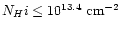 (Fig. 8).
When
is averaged over all the measured values,
(Fig. 8).
When
is averaged over all the measured values,
 at z < 3.1 is larger than
 at
.
Due to the lower
at
,
it
also seems clear from Fig. 8 that
gas at lower overdensities is
cooler at z < 3.1 than at higher z(keep in mind that a fixed column density corresponds
to a larger gas overdensity as z decreases due to the Hubble
expansion).
at
.
Due to the lower
at
,
it
also seems clear from Fig. 8 that
gas at lower overdensities is
cooler at z < 3.1 than at higher z(keep in mind that a fixed column density corresponds
to a larger gas overdensity as z decreases due to the Hubble
expansion).
If we assume Eq. (7) again and
 for
thermally broadened lines,
for
thermally broadened lines,
 .
When this simple conversion law is assumed,
.
When this simple conversion law is assumed,
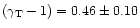 at z < 3.1 and
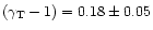 at
.
These
at
.
These
 could be considered to be
consistent with the results by McDonald et al.
(2000) within their error bars, although their
error bars at z =3.9 (
could be considered to be
consistent with the results by McDonald et al.
(2000) within their error bars, although their
error bars at z =3.9 (
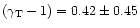 )
and at z=3 (
)
and at z=3 (
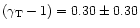 )
are rather large.
Their
)
are rather large.
Their
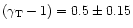 at
at
 agrees with our
 .
Our
is marginally in agreement
with the results from Ricotti et al. (2000)
and from Schaye et al. (2000).
Their
values are lower
at
and higher at
,
but within the error
bars.
.
Our
is marginally in agreement
with the results from Ricotti et al. (2000)
and from Schaye et al. (2000).
Their
values are lower
at
and higher at
,
but within the error
bars.
While the one-point function of the flux is more closely related
to observations, the one-point function of the optical depth
is usually calculated in simulations (Zhang et al. 1998;
Machacek et al. 2000). In the simulation by
Machacek et al. (2000), the H I optical depth  at which
the maximum
at which
the maximum
 occurs,
 ,
is
,
is
 at z=4,
 at z=3,
and
at z=3,
and
 at z=2.
Figure 22 shows
as a function of ,
which is calculated from the observed spectra at z < 2.4and the spectra generated
with noise at z > 2.4. The
value is
at z=2.
Figure 22 shows
as a function of ,
which is calculated from the observed spectra at z < 2.4and the spectra generated
with noise at z > 2.4. The
value is
 at
,
at
,
 at
at
 ,
and
,
and
 at
at
 ,
respectively.
The observed
shows a behavior similar
to the simulated results by Machacek et al. (2000).
However,
converges to
,
respectively.
The observed
shows a behavior similar
to the simulated results by Machacek et al. (2000).
However,
converges to
 at z < 2.4, not showing any z-dependence. Also there is
no z-dependence of
at
at z < 2.4, not showing any z-dependence. Also there is
no z-dependence of
at
 and at
z < 3.1.
and at
z < 3.1.
The optical depth
corresponds to
 ,
while
corresponds to
,
while
corresponds to
 ,
almost to the continuum level.
As z decreases, the number of pixels
with F = 0.96-0.99 increases. These pixels are
noise-dominated by the limited S/N and the continuum
fitting uncertainty.
Therefore, instead of showing
the expected z-dependence of
and
,
the observed
and
approach to
an asymptotic
,
almost to the continuum level.
As z decreases, the number of pixels
with F = 0.96-0.99 increases. These pixels are
noise-dominated by the limited S/N and the continuum
fitting uncertainty.
Therefore, instead of showing
the expected z-dependence of
and
,
the observed
and
approach to
an asymptotic
 value at z < 2.4and an asymptotic
at
and at z < 3.1, respectively.
value at z < 2.4and an asymptotic
at
and at z < 3.1, respectively.
At
 (or
0.05 < F < 0.9),
the observed
is simply
a different way of viewing the one-point function of the flux.
As z decreases,
decreases due to the expansion
of the universe. At
(or
0.05 < F < 0.9),
the observed
is simply
a different way of viewing the one-point function of the flux.
As z decreases,
decreases due to the expansion
of the universe. At  (or F < 0.05),
starts to converge again since it typically samples saturated regions, again
dominated by noise.
(or F < 0.05),
starts to converge again since it typically samples saturated regions, again
dominated by noise.
![\begin{figure}
\par\includegraphics[width=8.2cm,clip]{H2407F22.eps}\end{figure}](/articles/aa/full/2001/27/aah2407/img491.gif) |
Figure 22:
The z-evolution of
as a function
of .
The
values are
calculated from the observed spectra at z < 2.4 and
from the spectra generated with noise at z > 2.4. |
| z |
 |
 |
 |
(
 ) ) |
(
 ) ) |
||
| 1.61 | 0.086 |  0.010 0.010 |
0.020 |
| 1.98 | 0.161 | 0.016 |
0.021 |
| 2.13 | 0.131 | 0.012 |
0.021 |
| 2.66 | 0.234 | 0.014 |
0.020 |
| 2.87 | 0.275 | 0.015 |
0.020 |
| 3.75 | 0.733 | 0.013 |
0.013 |
We derived the baryon density,
 ,
from two
properties of the Ly
forest,
(including all the Ly
forest regardless of
)
and P(F) (only for
the forest with
,
from two
properties of the Ly
forest,
(including all the Ly
forest regardless of
)
and P(F) (only for
the forest with
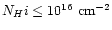 ).
).
If
 ,
the lower limits on the
baryon density become
,
the lower limits on the
baryon density become

Table 9 lists the lower limits on
at different z, together with the parameter values
used for calculating
 .
It should be noted that
the temperature used to
calculate Eq. (8) is smaller than the
values derived in Sect. 6.2, but in the present discussion
we are only interested in the lower
bounds on
.
These lower limits on
are consistent with
.
It should be noted that
the temperature used to
calculate Eq. (8) is smaller than the
values derived in Sect. 6.2, but in the present discussion
we are only interested in the lower
bounds on
.
These lower limits on
are consistent with
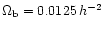 from the Big Bang
nucleosynthesis analysis (Copi et al. 1995). These
values also indicate that about 90% of all baryons reside
in the Ly
forest at
1.5 < z < 4.
from the Big Bang
nucleosynthesis analysis (Copi et al. 1995). These
values also indicate that about 90% of all baryons reside
in the Ly
forest at
1.5 < z < 4.
The lower bounds on the density parameter from the one-point
function,
 ,
are given by Weinberg et al. (1997) as
,
are given by Weinberg et al. (1997) as
![\begin{eqnarray*}\Omega_{\rm b}^{P(F)} & \ge & 0.021 h^{-3/2}\!\! \left(\!
\frac...
...{\gamma}} P(F)\,
{\rm d}F/F]^{\beta_{\gamma}/2}}{0.70}
\!\right)
\end{eqnarray*}](/articles/aa/full/2001/27/aah2407/img511.gif)
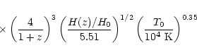
 ,
where
,
where
 is the power law index of the equation of state
(Weinberg et al. 1997).
is the power law index of the equation of state
(Weinberg et al. 1997).
Table 9 lists the lower bounds on
along with the
parameter values used to calculate
.
The
values are larger than
since
is not the true mean H I
opacity, but the effective opacity which underestimates
the true opacity when absorption lines become saturated.
The lower
limits from
P(F) are about a factor
of
 larger than
the Big Bang nucleosynthesis analysis,
.
larger than
the Big Bang nucleosynthesis analysis,
.
Our new lower bounds on
are a factor of
1.5 smaller than some of the previous results,
 -
-
 (Rauch et al. 1997;
Zhang et al. 1998; Burles et al. 1999;
Kirkman et al. 2000;
McDonald et al. 2000),
but still consistent with them within the error bars.
However, our lower
bounds are
not consistent with the derived
(Rauch et al. 1997;
Zhang et al. 1998; Burles et al. 1999;
Kirkman et al. 2000;
McDonald et al. 2000),
but still consistent with them within the error bars.
However, our lower
bounds are
not consistent with the derived
 -
-
 from the high D/H measurements
(Songaila et al. 1994; Rugers & Hogan 1996).
from the high D/H measurements
(Songaila et al. 1994; Rugers & Hogan 1996).
Copyright ESO 2001
![\begin{displaymath}N_H{\sc i} \sim \left[0.05\, (1+\delta) \,
10^{0.4 \,z}\right]^{1.43} \times 10^{14} \
{\rm cm}^{-2}.
\end{displaymath}](/articles/aa/full/2001/27/aah2407/img454.gif)
![\begin{figure}
\par\includegraphics[width=7.4cm,clip]{H2407F21.eps}\end{figure}](/articles/aa/full/2001/27/aah2407/img476.gif)
 errors. In the third panel,
error bars in the x-axis represent the z ranges over which
the median b values were estimated. Solid
lines represent the median
b values over
errors. In the third panel,
error bars in the x-axis represent the z ranges over which
the median b values were estimated. Solid
lines represent the median
b values over

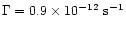 (at
(at
 ),
),
 (at
(at 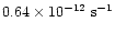 (at
(at
 (Haardt & Madau
 ,
and
,
and
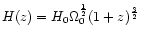 (Haardt & Madau