

 distribution
 forest
In addition to the three QSOs observed with UVES,
we have used the published line lists
of three QSOs at higher redshift observed
with similar resolution and S/N.
Table 2 lists all the analyzed QSOs
with their properties and the relevant references.
We have avoided a region close to
a damped Ly
system in the spectrum of Q0000-263
and a lower S/N region in the spectrum
of HS 1946+7658. The spectrum of Q0302-003
does not include the region of the known void at
 (cf. Dobrzycki & Bechtold 1991).
The fitted line parameters with the associated errors
of HS 1946+7658 and Q0000-263
were generated by VPFIT with a
(cf. Dobrzycki & Bechtold 1991).
The fitted line parameters with the associated errors
of HS 1946+7658 and Q0000-263
were generated by VPFIT with a  threshold of
 and
and
 ,
respectively.
The line list of Q0302-003
was generated by an automatized version of
the Voigt profile fitting program by Hu et al. (1995)
with
,
respectively.
The line list of Q0302-003
was generated by an automatized version of
the Voigt profile fitting program by Hu et al. (1995)
with
 and the errors associated with the fitted parameters
are not published.
and the errors associated with the fitted parameters
are not published.
The results of profile fitting are known to be sensitive to the data
quality as well as to the characteristics of the fitting program.
As a consequence, comparing line lists obtained with different criteria
is not usually straightforward.
Due to the use of a different fitting program,
the line list of Q0302-003 at
 should be
treated with caution
when combined with other line lists. A systematic difference in
b and
should be
treated with caution
when combined with other line lists. A systematic difference in
b and
 from VPFIT can introduce a slightly different
behavior of the Ly
forest at
.
While the
difference would not change the study of the line number
density or the correlation function significantly, it can affect
the determination of a lower cutoff b envelope in
the
-b diagrams.
Furthermore, the six QSOs in Table 2
cover the Ly
forest at
from VPFIT can introduce a slightly different
behavior of the Ly
forest at
.
While the
difference would not change the study of the line number
density or the correlation function significantly, it can affect
the determination of a lower cutoff b envelope in
the
-b diagrams.
Furthermore, the six QSOs in Table 2
cover the Ly
forest at
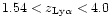 with a fairly regular spacing.
There is very little overlap between the Ly
forests of the different QSOs and the effects
of cosmic variance in the individual lines of sight might be important.
with a fairly regular spacing.
There is very little overlap between the Ly
forests of the different QSOs and the effects
of cosmic variance in the individual lines of sight might be important.
| QSO |
 |
 |
 |
d
 |
| HE 0515-4414 | 1.719 | 3090-3260 | 1.54-1.68 | 0.365 |
J2233-606
 |
2.238 | 3400-3850 | 1.80-2.17 | 1.104 |
| HE 2217-2818 | 2.413 | 3550-4050 | 1.92-2.33 | 1.286 |
HS 1946+7658
 |
3.051 | 4252-4635 | 2.50-2.81 | 1.157 |
Q0302-003
 |
3.290 | 4410-5000 | 2.63-3.11 | 1.878 |
Q0000-263
 |
4.127 | 5450-6100 | 3.48-4.02 | 2.540 |
The differential density distribution function,
 ,
is defined as the number of absorption lines per unit absorption
distance path
and per unit column density as a function of
(equivalent to the luminosity function of galaxies).
The absorption distance path X(z) is defined as
,
is defined as the number of absorption lines per unit absorption
distance path
and per unit column density as a function of
(equivalent to the luminosity function of galaxies).
The absorption distance path X(z) is defined as
![$X(z)
\equiv {1\over 2}
[(1+z)^{2} -1]$](/articles/aa/full/2001/27/aah2407/img105.gif) for
for
 or as
or as
![$X(z) \equiv {2\over 3}
[(1+z)^{3/2} -1]$](/articles/aa/full/2001/27/aah2407/img106.gif) for
for
 .
We used
for dX to compare our
with
the published
from the literature
(Table 2
lists the values of dX for
).
Empirically,
is fitted by a power law:
.
We used
for dX to compare our
with
the published
from the literature
(Table 2
lists the values of dX for
).
Empirically,
is fitted by a power law:
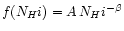 .
.
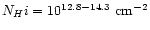
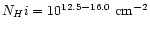
Figure 4 shows the observed
 as a function of
 for different redshifts.
The dotted line represents
the incompleteness-corrected
at
for different redshifts.
The dotted line represents
the incompleteness-corrected
at
 from Hu et al. (1995),
i.e.
from Hu et al. (1995),
i.e.
 .
Note that the apparent flattening of the slope towards
lower column densities in the observed
-
diagram is caused by line blending and limited S/N, i.e. incompleteness, which
becomes more severe at higher z.
For incompleteness-corrected
at z > 2.5 (Hu et al. 1995; Lu et al. 1996;
Kim et al. 1997), this apparent flattening disappears.
The incompleteness-corrected
at
over
.
Note that the apparent flattening of the slope towards
lower column densities in the observed
-
diagram is caused by line blending and limited S/N, i.e. incompleteness, which
becomes more severe at higher z.
For incompleteness-corrected
at z > 2.5 (Hu et al. 1995; Lu et al. 1996;
Kim et al. 1997), this apparent flattening disappears.
The incompleteness-corrected
at
over
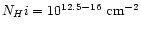 is similar to the incompleteness-corrected
at
is similar to the incompleteness-corrected
at
 (Lu et al. 1996) and
at
(Lu et al. 1996) and
at
 (Kim et al. 1997) over the same column density
range.
The amount of
incompleteness extrapolated from at z > 2.5 (Hu et al. 1995;
Lu et al. 1996;
Kim et al. 1997; Kirkman & Tytler 1997)
becomes negligible at z < 2.4 and we assume the observed
as representative of the actual
at z < 2.4.
(Kim et al. 1997) over the same column density
range.
The amount of
incompleteness extrapolated from at z > 2.5 (Hu et al. 1995;
Lu et al. 1996;
Kim et al. 1997; Kirkman & Tytler 1997)
becomes negligible at z < 2.4 and we assume the observed
as representative of the actual
at z < 2.4.
In the column density range
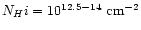 ,
the observed
at z < 2.4 is in
good agreement for the different QSOs
and also agrees
with the incompleteness-corrected
at
2.6< z < 4.0.
This suggests that there is very little
evolution in
in the interval
1.5 <z < 4for forest lines with
.
At
,
the observed
at z < 2.4 is in
good agreement for the different QSOs
and also agrees
with the incompleteness-corrected
at
2.6< z < 4.0.
This suggests that there is very little
evolution in
in the interval
1.5 <z < 4for forest lines with
.
At
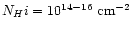 ,
shows differences at different z. Kim et al. (1997) noted
that at lower z,
starts to deviate from a single power
law for
,
shows differences at different z. Kim et al. (1997) noted
that at lower z,
starts to deviate from a single power
law for
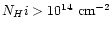 and that the column density at which the deviation
from a single power-law starts
decreases as z decreases. The deviation from the single power-law
in
is evident in Fig. 4.
While the forest at
is still well approximated by a single
power-law over
,
the forest at z<2.4 starts to deviate from the power law
at
and that the column density at which the deviation
from a single power-law starts
decreases as z decreases. The deviation from the single power-law
in
is evident in Fig. 4.
While the forest at
is still well approximated by a single
power-law over
,
the forest at z<2.4 starts to deviate from the power law
at
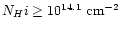 with a
decreasing number of lines at
.
with a
decreasing number of lines at
.
Table 3 lists the parameters of a
maximum-likelihood power-law fit to various column density ranges.
These column density ranges are selected for comparison with
the previous observational results of Kim et al. (1997)
and Penton et al. (2000) and with simulations of
Zhang et al. (1998) and Machacek et al. (2000).
At
 ,
the slope
,
the slope  is
approximately 1.4 in the interval
and 1.68 in the interval
,
i.e. the slope is steeper for
higher column density clouds. At
is
approximately 1.4 in the interval
and 1.68 in the interval
,
i.e. the slope is steeper for
higher column density clouds. At
 ,
the slopes
,
the slopes
 -1.72 are steeper
for both column density ranges.
This indicates that the slope of
increases from
to
-1.72 are steeper
for both column density ranges.
This indicates that the slope of
increases from
to
 .
Assuming a curve of growth with
.
Assuming a curve of growth with
 km s-1,
Penton et al. (2000) found that the slope of
at
km s-1,
Penton et al. (2000) found that the slope of
at
 over
and over
is
over
and over
is
 and
and
 ,
respectively.
The slopes over
are steeper at
and at
than
at z > 1.8, and suggest that the incompleteness correction at
z > 1.8 might be underestimated or that the slope becomes
intrinsically steeper at z < 1.8.
The slopes over
,
respectively.
The slopes over
are steeper at
and at
than
at z > 1.8, and suggest that the incompleteness correction at
z > 1.8 might be underestimated or that the slope becomes
intrinsically steeper at z < 1.8.
The slopes over
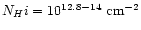 and
are
in agreement with the ones found by Kim et al. (1997)
at
and
are
in agreement with the ones found by Kim et al. (1997)
at
 .
However,
our measurement of
.
However,
our measurement of
 at
(only from
HE 2217-2818 and J2233-606)
over
at
(only from
HE 2217-2818 and J2233-606)
over
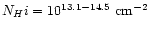 is lower than the previous determination of
 over the
same column density range
at
over the
same column density range
at
 by Kulkarni et al. (1996).
While these observed
values at
1.5 < z < 2.4 can be
obtained with
semi-analytic models by Hui et al. (1997),
they are lower than the values predicted
from numerical simulations
(Zhang et al. 1998; Machacek et al. 2000),
by more than
 .
The slope depends on the
amplitude of the power spectrum and models with less power
produce steeper slopes. Thus, the steeper slopes from the simulations
by Zhang et al. (1998) and Machacek et al. (2000)
suggest that their index for the power spectrum,
.
The slope depends on the
amplitude of the power spectrum and models with less power
produce steeper slopes. Thus, the steeper slopes from the simulations
by Zhang et al. (1998) and Machacek et al. (2000)
suggest that their index for the power spectrum,
 ,
might be smaller than the actual index of the power spectrum.
,
might be smaller than the actual index of the power spectrum.
The line number density per unit redshift is defined as dn/dz =
(dn/d
 ,
where
(dn/d
,
where
(dn/d is the
local comoving number density of the forest. For a non-evolving
population in the standard Friedmann universe with the cosmological constant
is the
local comoving number density of the forest. For a non-evolving
population in the standard Friedmann universe with the cosmological constant

![[*]](/icons/foot_motif.gif) ,
,
 and 0.5 for
and 0.5,
respectively. In practice, the measured
and 0.5 for
and 0.5,
respectively. In practice, the measured  is dependent on the
chosen column density interval, the redshift and the spectral
resolution. Therefore, comparisons between individual studies
are complicated (Kim et al. 1997).
is dependent on the
chosen column density interval, the redshift and the spectral
resolution. Therefore, comparisons between individual studies
are complicated (Kim et al. 1997).
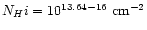
Figure 5 shows the number density evolution of the
Ly
forest in the interval
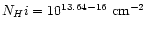 .
This range has been chosen to allow a
comparison with the HST results from the HST QSO absorption
line Key Project at z < 1.5 from Weymann et al.
(1998), for which a threshold in
the equivalent width of 0.24 Å was adopted.
We assumed the conversion between the equivalent width and
the column density to be
.
This range has been chosen to allow a
comparison with the HST results from the HST QSO absorption
line Key Project at z < 1.5 from Weymann et al.
(1998), for which a threshold in
the equivalent width of 0.24 Å was adopted.
We assumed the conversion between the equivalent width and
the column density to be
 ,
where W is the equivalent width in
angstrom,
,
where W is the equivalent width in
angstrom,
 is the wavelength of Ly
in
angstrom, f is the oscillator strength of Ly(Cowie & Songaila 1986).
The value of the square (Penton et al. 2000)
was estimated under the assumption of b=25 km s-1 from
the equivalent widths (corresponding to the column density range
is the wavelength of Ly
in
angstrom, f is the oscillator strength of Ly(Cowie & Songaila 1986).
The value of the square (Penton et al. 2000)
was estimated under the assumption of b=25 km s-1 from
the equivalent widths (corresponding to the column density range
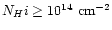 )
and is lower than
the extrapolated dn/dz at
)
and is lower than
the extrapolated dn/dz at
 from the Weymann et al.
results, but within the error bar.
Pentagons (Savaglio et al. 1999 from the line fitting
analysis) also correspond to the column density range
.
Note that
from W depends on an assumed b parameter,
resolution and S/N.
Also note that
including lines with
from the Weymann et al.
results, but within the error bar.
Pentagons (Savaglio et al. 1999 from the line fitting
analysis) also correspond to the column density range
.
Note that
from W depends on an assumed b parameter,
resolution and S/N.
Also note that
including lines with
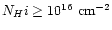 from line fitting analyses
introduces a further uncertainty on the line counting since different
programs deblend completely saturated lines differently,
resulting in different
numbers of lines for the same saturated lines.
from line fitting analyses
introduces a further uncertainty on the line counting since different
programs deblend completely saturated lines differently,
resulting in different
numbers of lines for the same saturated lines.
The long-dashed line is the maximum-likelihood fit
to the UVES and the HIRES data at z > 1.5:
dn/d
 .
This
is lower than previously reported
.
This
is lower than previously reported
 (Lu et al. 1991; Kim et al.
1997).
This slope is steeper than the expected values for the non-evolving
forest for a universe with
(Lu et al. 1991; Kim et al.
1997).
This slope is steeper than the expected values for the non-evolving
forest for a universe with
 ,
,
 and
and
 .
These results suggest that the Ly
forest at
.
These results suggest that the Ly
forest at
 evolves and that
its evolution
slows down as z decreases.
Interestingly, the HST data point at
evolves and that
its evolution
slows down as z decreases.
Interestingly, the HST data point at
 (the open
triangle at the boundary of the shaded area), which has been measured
in the line-of-sight to the QSO UM 18 and was
suggested to be an outlier by Weymann et al. (1998), is
now in good agreement with the extrapolated fit from higher z.
(the open
triangle at the boundary of the shaded area), which has been measured
in the line-of-sight to the QSO UM 18 and was
suggested to be an outlier by Weymann et al. (1998), is
now in good agreement with the extrapolated fit from higher z.
Despite the different line counting methods between the HST observations
(based on the equivalent width)
and the high-resolution observations
(based on the profile fitting), a change of the slope in the Lynumber density does seem to be real. The
UVES observations suggest that the slow-down in the evolution does occur
at
 ,
rather than at
,
rather than at
 as previously suggested
(Impey et al. 1996; Weymann et al. 1998),
although the different methods of line counting at higher and lower
z make it a little uncertain.
At least, down to
as previously suggested
(Impey et al. 1996; Weymann et al. 1998),
although the different methods of line counting at higher and lower
z make it a little uncertain.
At least, down to
 ,
the number density of the forest evolves as
at higher z, which suggests that any major drive governing the
forest evolution at z > 2 continues to dominate the forest evolution
down to
.
Since the Hubble expansion is the main
drive
governing the forest evolution at z > 2 (Miralda-Escudé et al.
1996), the continuously decreasing number density of
the forest down to
implies that the Hubble expansion
continues to dominate the forest evolution down to
.
,
the number density of the forest evolves as
at higher z, which suggests that any major drive governing the
forest evolution at z > 2 continues to dominate the forest evolution
down to
.
Since the Hubble expansion is the main
drive
governing the forest evolution at z > 2 (Miralda-Escudé et al.
1996), the continuously decreasing number density of
the forest down to
implies that the Hubble expansion
continues to dominate the forest evolution down to
.
![\begin{figure}
\par\includegraphics[width=7.8cm,clip]{H2407F5.eps}\end{figure}](/articles/aa/full/2001/27/aah2407/img193.gif) |
Figure 5:
The number density evolution of the Ly
forest.
The column density range
has been chosen
to allow a comparison with the HST results
from Weymann et al. (1998),
which are shown as open triangles.
Filled symbols are estimated from HE 0515-4414
at
 ,
from J2233-606 at ,
from J2233-606 at
 and from HE 2217-2818 at
 ,
respectively.
The star, open circles, and the diamond are taken
from the HIRES data at similar resolutions by Lu et al.
(1996),
Kim et al. (1997), and Kirkman & Tytler (1997),
respectively.
The square and pentagons are taken from Penton et al.
(2000) and Savaglio et al. (1999), respectively,
over
.
Horizontal solid lines represent the z interval over which
the number density was estimated. Vertical solid lines represent
the ,
respectively.
The star, open circles, and the diamond are taken
from the HIRES data at similar resolutions by Lu et al.
(1996),
Kim et al. (1997), and Kirkman & Tytler (1997),
respectively.
The square and pentagons are taken from Penton et al.
(2000) and Savaglio et al. (1999), respectively,
over
.
Horizontal solid lines represent the z interval over which
the number density was estimated. Vertical solid lines represent
the  Poisson errors.
The shaded area is the z range where UVES is extremely
sensitive.
The long-dashed line is the maximum likelihood fit to the UVES and
the HIRES data at z > 1.5.
The UVES observations indicate that the number density evolution
of the Ly
forest at z > 2.4 continues at least
down to
and that a slope change occurs at
.
Poisson errors.
The shaded area is the z range where UVES is extremely
sensitive.
The long-dashed line is the maximum likelihood fit to the UVES and
the HIRES data at z > 1.5.
The UVES observations indicate that the number density evolution
of the Ly
forest at z > 2.4 continues at least
down to
and that a slope change occurs at
. |
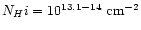
Figure 6 is similar to Fig. 5,
except for the
range:
 .
The correction for incompleteness due to line blending
is still negligible in this column density range
(Fig. 4 shows that the number of lines per unit
column density over
is still well represented by a single power-law).
Again, the square from Penton et al. (2000) is estimated
from the equivalent widths with the assumed b=25 km s-1.
The dot-dashed line is the maximum-likelihood fit to the lower column
density forest of the UVES and the HIRES data:
dn/d
.
The correction for incompleteness due to line blending
is still negligible in this column density range
(Fig. 4 shows that the number of lines per unit
column density over
is still well represented by a single power-law).
Again, the square from Penton et al. (2000) is estimated
from the equivalent widths with the assumed b=25 km s-1.
The dot-dashed line is the maximum-likelihood fit to the lower column
density forest of the UVES and the HIRES data:
dn/d
 .
At
2.4 < z < 4 and at
2.1 < z < 4,
.
At
2.4 < z < 4 and at
2.1 < z < 4,
 and
and
 ,
respectively.
For the column density range
,
the forest does not show any strong evolution.
,
respectively.
For the column density range
,
the forest does not show any strong evolution.
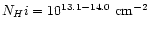
Note that the point at
 (diamond)
from Kirkman & Tytler (1997) indicates
a number density twice as large as than at
(diamond)
from Kirkman & Tytler (1997) indicates
a number density twice as large as than at
 in the interval
 (excluding the
forest, the maximum-likelihood
fit becomes dn/d
(excluding the
forest, the maximum-likelihood
fit becomes dn/d
 ).
Although this discrepancy could result from a real cosmic variance of
the number density from sightline to sightline,
the number density in the interval
).
Although this discrepancy could result from a real cosmic variance of
the number density from sightline to sightline,
the number density in the interval
 from the same line of sight is in good agreement with
other HIRES data. The differential
density distribution function (Fig. 4) and the mean H I
opacity (Fig. 15) towards this line of sight suggest that
the discrepancy at
is due to overfitting, which, as discussed in Sect. 3, may occur
especially in high S/N data.
from the same line of sight is in good agreement with
other HIRES data. The differential
density distribution function (Fig. 4) and the mean H I
opacity (Fig. 15) towards this line of sight suggest that
the discrepancy at
is due to overfitting, which, as discussed in Sect. 3, may occur
especially in high S/N data.
As previously noticed (Kim et al. 1997),
the lower column density forest evolves at a slower rate
than the higher
column density forest. The evolutionary rate
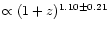 would be consistent with no evolution for
 or
mild evolution for
.
For
,
and
,
the Ly
forest with
is mildly evolving
at z > 1.5.
The Ly
forest with
appears
more numerous at
or
mild evolution for
.
For
,
and
,
the Ly
forest with
is mildly evolving
at z > 1.5.
The Ly
forest with
appears
more numerous at  than
expected when extrapolating from the z > 1.5 range.
than
expected when extrapolating from the z > 1.5 range.
![\begin{figure}
\par\includegraphics[width=7.8cm,clip]{H2407F6.eps}\end{figure}](/articles/aa/full/2001/27/aah2407/img208.gif) |
Figure 6:
The number density evolution of the Ly
forest at
the
range
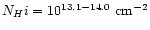 .
Symbols are the same as in Fig. 5.
The dot-dashed line (solid line)
is the maximum likelihood fit to the lower column
density forest including the .
Symbols are the same as in Fig. 5.
The dot-dashed line (solid line)
is the maximum likelihood fit to the lower column
density forest including the  = 2.66 forest (excluding
the
= 2.66 forest),
while the dashed line represents the maximum
likelihood fit to the forest at
from
Fig. 5.
= 2.66 forest (excluding
the
= 2.66 forest),
while the dashed line represents the maximum
likelihood fit to the forest at
from
Fig. 5. |
distribution
 parameter
For a photoionized gas,
a temperature-density relation exists, i.e. the equation of state:
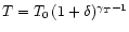 ,
where T is the gas temperature, T0 is the gas temperature
at the mean gas density,
,
where T is the gas temperature, T0 is the gas temperature
at the mean gas density,  is the baryon overdensity,
 (
(
 is the mean baryon density), and
 is a constant which depends on the reionization history
(Hui & Gnedin 1997).
For an abrupt reionization at
is a constant which depends on the reionization history
(Hui & Gnedin 1997).
For an abrupt reionization at  ,
the temperature of the mean gas
density decreases as z decreases after the reionization,
eventually approaching an asymptotic
,
the temperature of the mean gas
density decreases as z decreases after the reionization,
eventually approaching an asymptotic  .
For a generally assumed
QSO-dominated UV background with a sudden turn-on of QSOs at
5 < z < 10,
T0 decreases as z decreases at 2 < z < 4(Hui & Gnedin 1997).
.
For a generally assumed
QSO-dominated UV background with a sudden turn-on of QSOs at
5 < z < 10,
T0 decreases as z decreases at 2 < z < 4(Hui & Gnedin 1997).
Under the assumption that there are
some lines which are broadened primarily by the thermal motion
at any given column density, this equation of state translates
into a lower cutoff
 envelope in the
-b distribution: T and
can be derived from b and
.
For the equation of state
envelope in the
-b distribution: T and
can be derived from b and
.
For the equation of state
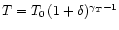 ,
,
 becomes
 is the intercept of the cutoff
in the
is the intercept of the cutoff
in the
 -
- diagram and
 is the slope of the cutoff
(Schaye et al. 1999).
The cutoff slope
is proportional
to
is the slope of the cutoff
(Schaye et al. 1999).
The cutoff slope
is proportional
to
 .
This cutoff envelope provides a probe of the gas temperature of the IGM
at a given z, thus giving a powerful constraint on the thermal
history of the IGM (Hu et al. 1995;
Lu et al. 1996; Kim et al. 1997;
Kirkman & Tytler 1997; Zhang et al. 1997;
Schaye et al. 1999;
Bryan & Machacek 2000; McDonald et al. 2000;
Ricotti et al. 2000;
Schaye et al. 2000).
.
This cutoff envelope provides a probe of the gas temperature of the IGM
at a given z, thus giving a powerful constraint on the thermal
history of the IGM (Hu et al. 1995;
Lu et al. 1996; Kim et al. 1997;
Kirkman & Tytler 1997; Zhang et al. 1997;
Schaye et al. 1999;
Bryan & Machacek 2000; McDonald et al. 2000;
Ricotti et al. 2000;
Schaye et al. 2000).
In practice, defining
in an objective manner is not trivial due
to the finite number of available absorption lines,
sightline-to-sightline
cosmic variances, limited S/N,
and unidentified metal lines.
Among several methods proposed to derive
,
we have adopted the following three:
the iterative power-law fit, the power-law fit
to the smoothed b distribution, and the b distribution.
We refer the reader to other papers for more methods
to derive
(Hu et al. 1995;
McDonald et al. 2000;
Theuns & Zaroubi 2000).
In our analysis, we divide the data points into 2 groups:
Sample A and Sample B.
Sample A consists of the lines in the range
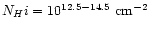 with errors less than 25% in both
and b
in order to avoid ill-fitted values from VPFIT.
Sample B consists of all the lines with
regardless of errors.
The criteria for Sample A and Sample B are chosen to compare our results with
the previous results
by Schaye et al. (2000) and to investigate whether it is
reasonable to include the Q0302-003 line list
for which
error estimates are not given. As no errors are
available for Q0302-003,
no Sample A can be defined at
.
Note that including
the relatively few lines
with
with errors less than 25% in both
and b
in order to avoid ill-fitted values from VPFIT.
Sample B consists of all the lines with
regardless of errors.
The criteria for Sample A and Sample B are chosen to compare our results with
the previous results
by Schaye et al. (2000) and to investigate whether it is
reasonable to include the Q0302-003 line list
for which
error estimates are not given. As no errors are
available for Q0302-003,
no Sample A can be defined at
.
Note that including
the relatively few lines
with
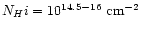 does not change
the results significantly.
There is hardly any overlap in z, except for
J2233-606 and HE 2217-2818. Since one of our
aims is to probe the z-evolution
of
,
we analyze the b distribution
of each line of sight individually to derive
.
does not change
the results significantly.
There is hardly any overlap in z, except for
J2233-606 and HE 2217-2818. Since one of our
aims is to probe the z-evolution
of
,
we analyze the b distribution
of each line of sight individually to derive
.
Since the equation of state is a power law, it is reasonable
to fit
- with one.
We did so, using the bootstrap method described by Schaye et al. (1999),
iterating until convergence was reached. After each iteration,
those points were excluded that lay more than one
mean absolute deviation above the fit.
Finally, the lines more
than one mean absolute deviation below the fit were also taken out
and the final power law fit,
with one.
We did so, using the bootstrap method described by Schaye et al. (1999),
iterating until convergence was reached. After each iteration,
those points were excluded that lay more than one
mean absolute deviation above the fit.
Finally, the lines more
than one mean absolute deviation below the fit were also taken out
and the final power law fit,
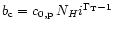 ,
was carried out.
The procedure was repeated over 200 bootstrap realizations in order to
determine the full probability distribution of the parameters of
the cutoff.
As noted by Schaye et al. (2000), the power law fit requires
over 200 available lines to reach stable fit parameters.
,
was carried out.
The procedure was repeated over 200 bootstrap realizations in order to
determine the full probability distribution of the parameters of
the cutoff.
As noted by Schaye et al. (2000), the power law fit requires
over 200 available lines to reach stable fit parameters.
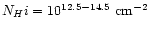
Figure 7 shows the iterative power law fit in the
-b distributions.
The noticeable difference between Sample A (cross symbols)
and Sample B (cross symbols and open circles)
occurs at
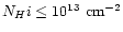 .
These lines
usually come from blends or from weak, asymmetric absorption lines.
Table 4 lists the fitted parameters, such as
.
These lines
usually come from blends or from weak, asymmetric absorption lines.
Table 4 lists the fitted parameters, such as
 and
,
including
values at the fixed column density
and
,
including
values at the fixed column density
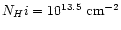 ,
,
 ,
for Sample A and Sample B.
,
for Sample A and Sample B.
The power law fit between Sample A
and Sample B does not give a significant difference except at
and at
 ,
for which
several lines with
,
for which
several lines with  km s-1and
contribute to a
different power law fit for Sample B.
This suggests that using the Q0302-003 line
list at
without error bars does not severely
distort our conclusions. Note that
the power law fit at
might be less steep
with a higher intercept,
if the same general behavior of errors also occurs for
the Q0302-003 forest (larger errors at
km s-1 or
km s-1and
contribute to a
different power law fit for Sample B.
This suggests that using the Q0302-003 line
list at
without error bars does not severely
distort our conclusions. Note that
the power law fit at
might be less steep
with a higher intercept,
if the same general behavior of errors also occurs for
the Q0302-003 forest (larger errors at
km s-1 or  km s-1).
Due to the small number of lines (47 lines for
Sample A and 56 lines for Sample B) at
,
the power law fit
should be taken as an upper limit on
and indeed it
provides the highest
among all the z bins.
For both Sample A and Sample B, there is a weak trend of
increasing
as z decreases, except at
which shows a higher
value than at the adjacent z ranges
(see Sect. 6.2 for further discussion).
On the other hand, the power law slope
is rather ill-defined with z with a possible
flatter slope at
than at z < 3.1.
km s-1).
Due to the small number of lines (47 lines for
Sample A and 56 lines for Sample B) at
,
the power law fit
should be taken as an upper limit on
and indeed it
provides the highest
among all the z bins.
For both Sample A and Sample B, there is a weak trend of
increasing
as z decreases, except at
which shows a higher
value than at the adjacent z ranges
(see Sect. 6.2 for further discussion).
On the other hand, the power law slope
is rather ill-defined with z with a possible
flatter slope at
than at z < 3.1.
Figure 8 shows the power law fit to Sample A
at
(small filled circles;
242 lines from J2233-606 and
HE 2217-28118)
and at
(open squares; 209 lines) over
(upper panel) and over
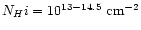 (lower panel).
The fitted parameters are given in Table 4.
For both
ranges,
the slopes of
are steeper
at
than at
.
This result, however, is certainly biased by the lack of
lines with
(lower panel).
The fitted parameters are given in Table 4.
For both
ranges,
the slopes of
are steeper
at
than at
.
This result, however, is certainly biased by the lack of
lines with  km s-1 and
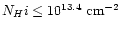 at higher z,
due to the severe line blending.
at higher z,
due to the severe line blending.
| Sample A | Sample B | ||||||||
|
#
 |
 |
|
(km
s-1)
|
#
|
|
|
(km s-1)
|
|
| 1.61 | 47 |
 |
 |
 |
56 |
 |
|
 |
|
| 1.98 | 103 |
 |
 |
 |
146 |
 |
 |
 |
|
| 2.13 | 139 |
 |
 |
 |
181 |
 |
 |
 |
|
| 2.66 | 140 |
 |
|
 |
204 |
 |
 |
 |
|
| 2.87 | - | - | - | - | 223 |
 |
 |
 |
|
| 3.75 | 209 |
 |
 |
 |
271 |
 |
 |
 |
|
| 2.1
|
242 |
 |
 |
 |
327 |
 |
|
 |
|
| 2.1
|
156 |
 |
|
 |
187 |
 |
|
 |
|
| 3.75
|
188 |
 |
|
 |
233 |
 |
|
 |
|
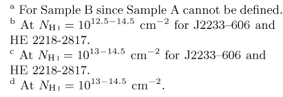
and the minimum/maximum
from the 200 bootstrap realizations for the given
-bpairs. The typical
of the
distribution
from the 200 bootstrap realizations is  0.3 kms-1, which is
underestimated (cf. Schaye et al. 2000).
.
.
.
0.3 kms-1, which is
underestimated (cf. Schaye et al. 2000).
.
.
.
![\begin{figure}
\par\includegraphics[width=7.7cm,clip]{H2407F8.eps}\end{figure}](/articles/aa/full/2001/27/aah2407/img287.gif) |
Figure 8:
The
-b diagrams with the power law
fits at
(only for J2233-606 and
HE 2217-2818; small filled circles) and at
(open squares).
At both redshifts, the data points with errors less than 25% in both
and b are displayed.
The upper panel shows the fit to the column density range
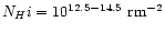 ,
while
the lower panel is to the range ,
while
the lower panel is to the range
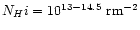 .
The vertical dotted lines in each panel represent the column density
range over which the power law fit was carried out.
The solid line shows the power law fit at
,
and the
dashed line at z=3.75.
A deficit of
lines with .
The vertical dotted lines in each panel represent the column density
range over which the power law fit was carried out.
The solid line shows the power law fit at
,
and the
dashed line at z=3.75.
A deficit of
lines with
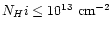 and kms-1observed at
is due in part to the fact
that all the fitted
lines with
and kms-1 have errors larger than
25% and in part to the severe line blending which
limits the detection of weak lines.
and kms-1observed at
is due in part to the fact
that all the fitted
lines with
and kms-1 have errors larger than
25% and in part to the severe line blending which
limits the detection of weak lines. |
Bryan & Machacek (2000) presented a method to measure
from a power law fit to
a smoothed b distribution, sorting absorption lines
by
and then dividing them into groups
containing similar numbers of lines.
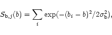
The b distribution in each group was then smoothed with a Gaussian filter with
a smoothing constant
 :
:
 |
(2) |
 is the smoothed density of lines in each group jand i indicates the lines in the group.
Then, the location of the first peak in the derivative of
defines the lower cutoff
at the average column density,
is the smoothed density of lines in each group jand i indicates the lines in the group.
Then, the location of the first peak in the derivative of
defines the lower cutoff
at the average column density,
 ,
for the jth group.
,
for the jth group.
Figure 9 shows the
-b diagram at each
z with the
points for each group (filled circles)
measured from the smoothed
b distributions.
We use the smoothing constant
 kms-1. However,
is largely insensitive to the smoothing constant.
In general, 30 lines were included in each group except
for the last group at higher
for which typically smaller
numbers of lines
were available.
For this same reason, at
groups of 16 lines were used.
The solid line represents the
robust least-squares power law fit
to filled circles:
kms-1. However,
is largely insensitive to the smoothing constant.
In general, 30 lines were included in each group except
for the last group at higher
for which typically smaller
numbers of lines
were available.
For this same reason, at
groups of 16 lines were used.
The solid line represents the
robust least-squares power law fit
to filled circles:
 .
Table 5 lists the parameters of
the power law fit to the smoothed bdistributions.
.
Table 5 lists the parameters of
the power law fit to the smoothed bdistributions.
We find that the power law fit to the smoothed b distribution
produces in general a lower intercept and a steeper slope
than the iterative power law fit. It also produces smaller
 values.
Direct comparison of Figs. 9 with 7
indicates that
measured
from the smoothed b distribution
can be considered as a lower limit on the real
,
while
from the
iterative power law fit can be considered as an upper limit
on the real
.
values.
Direct comparison of Figs. 9 with 7
indicates that
measured
from the smoothed b distribution
can be considered as a lower limit on the real
,
while
from the
iterative power law fit can be considered as an upper limit
on the real
.
As with the iterative power law fit,
measured from the smoothed b distribution
increases continuously as z decreases,
except at
,
where
is higher than at the adjacent redshifts
(see Sect. 6.2 for further discussion).
The slope
measured from the smoothed b distribution
also does not show any well-defined trend with
z.
|
|
 |
|
|
| (km s-1) | |||
| 1.61 |
 |
 |
 |
| 1.98 |
 |
 |
 |
| 2.13 |
 |
 |
 |
| 2.66 |
 |
 |
 |
| 2.87
|
 |
 |
 |
| 3.75 |
 |
 |
 |
| 2.1
|
 |
 |
 |
| 2.1
|
 |
 |
 |
| 3.75
|
 |
 |
 |
distributions
Assuming that absorption lines arise from
local optical depth ( )
peaks and that
)
peaks and that  is a Gaussian random
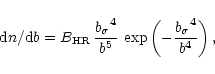
variable, Hui & Rutledge (1999) derived a single-parameter b
distribution:
is a Gaussian random
variable, Hui & Rutledge (1999) derived a single-parameter b
distribution:
 |
(3) |
 is a
constant and
is a
constant and
 is a parameter determined by the average amplitude of the fluctuations and the
effective smoothing scale.
is a parameter determined by the average amplitude of the fluctuations and the
effective smoothing scale.
Figure 10 shows the observed b distributions
at each z. The
noticeable difference between Sample A (solid lines) and
Sample B (dot-dashed lines)
occurs at
km s-1 or
km s-1.
These spurious lines are usually introduced by VPFIT
to fit the noise so that the overall profile of H I forest complexes
could be improved.
The dashed line represents
the best-fitting Hui-Rutledge b distribution, while
the dotted line represents the b parameter for which
the Hui-Rutledge b distribution function vanishes
to 10-4,
 ,
i.e.
the truncated b value for the Hui-Rutledge bdistribution function.
The parameter
cannot be considered equivalent to
the cutoff since it is derived from the b distribution
without assuming the
dependence on
.
It is more sensitive to smaller b values in the b distribution,
which are in general coupled with lower
.
Table 6 lists the relevant parameters describing
the Hui-Rutledge b distribution for Sample A,
such as the constant
,
,
i.e.
the truncated b value for the Hui-Rutledge bdistribution function.
The parameter
cannot be considered equivalent to
the cutoff since it is derived from the b distribution
without assuming the
dependence on
.
It is more sensitive to smaller b values in the b distribution,
which are in general coupled with lower
.
Table 6 lists the relevant parameters describing
the Hui-Rutledge b distribution for Sample A,
such as the constant
,
 ,
and the
median b values at different column density ranges.
,
and the
median b values at different column density ranges.
It is hard to specify subtle differences among the bdistributions: while the modal b value and the
value
have a
minimum at
,
they have a maximum at
.
The
forest
also has the broadest b distribution. However, this large  could be in part due to a different fitting program
and in part due to a lack of information on the errors.
Other parameters, such as
,
,
and
,
appear to be fairly constant
with z.
could be in part due to a different fitting program
and in part due to a lack of information on the errors.
Other parameters, such as
,
,
and
,
appear to be fairly constant
with z.
![\begin{figure}
\par\includegraphics[width=7.9cm,clip]{H2407F11.eps}\end{figure}](/articles/aa/full/2001/27/aah2407/img331.gif) |
Figure 11:
The b distribution as a function of z for Sample A
(Sample B at
).
The horizontal
dashed line indicates b = 20 kms-1 which is a
-independent at
(Hu et al. 1995).
Circles, crosses, diamonds, stars,
triangles and squares are from HE 0515-4414,
J2233-606, HE 2217-2818, HS 1946+7658,
Q0302-003 and Q0000-263, respectively.
There is an indication of increasing
with decreasing
z at
.
At z < 3.1,
is not clearly
defined. |
Figure 11
shows the b distribution with z. This diagram
does not assume a
dependence on
,
but is sensitive to a local
variance.
At z < 3.1,
there is no clear indication
of the behavior of the lower cutoff b values as a function of z.
However, there is
a clear indication of a trend with z of the lower cutoff b
values over
3.5 < z < 3.9.
In Fig. 11, there are distinct regions at
1.8 < z < 2.4.
The apparent cutoff values in b at
2.2 < z < 2.4 and at
1.8 < z < 1.9are clearly higher than at
1.9 < z < 2.2. The
2.2 < z < 2.4 region towards HE 2217-2818
corresponds to a 44 Mpc void (the region
B in Fig. 14), which might suggest enhanced
ionization due to a nearby QSO or processes of
galaxy formation (Theuns et al. 2000a).
Mpc void (the region
B in Fig. 14), which might suggest enhanced
ionization due to a nearby QSO or processes of
galaxy formation (Theuns et al. 2000a).
|
|
|
|
|
 |
 |
| (km s-1) | (km s-1) | (km s-1) | (km s-1) | ||
| 1.61 | 7.37 | 23.01 | 12.61 | 28.14 | 34.56 |
| 1.98 | 7.98 | 23.83 | 13.04 | 26.04 | 29.10 |
| 2.13 | 7.46 | 23.61 | 12.95 | 25.34 | 29.57 |
| 2.66 | 6.82 | 24.09 | 13.25 | 28.30 | 30.10 |
| 2.87 | 7.09 | 27.75 | 15.30 | 28.74 | 34.05 |
| 3.75 | 6.72 | 22.41 | 12.31 | 28.90 | 30.70 |
from Sample A (Sample B at
).
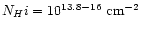 from Sample A (Sample B at
).
from Sample A (Sample B at
).
The Ly
forest contains information on the large-scale matter
distribution and the simplest way to study it is to compute the
two-point velocity correlation function,
 .
The correlation function compares the observed
number of pairs (
.
The correlation function compares the observed
number of pairs (
 )
with the expected number of pairs
(
)
with the expected number of pairs
(
 )
from a random distribution in a given velocity bin
(
)
from a random distribution in a given velocity bin
( ):
):
 ,
where
,
where
![$\Delta v = c\,(z_{2}-z_{1})/[1+ (z_{2}+z_{1})/2]$](/articles/aa/full/2001/27/aah2407/img340.gif) ,
z1 and z2 are redshifts of two lines and c is the
speed of light (Cristiani et al. 1995; Cristiani et al. 1997;
Kim et al. 1997).
,
z1 and z2 are redshifts of two lines and c is the
speed of light (Cristiani et al. 1995; Cristiani et al. 1997;
Kim et al. 1997).
Studies of the correlation function of the Ly
forest have
generally led to conflicting results even at similar z. Some
studies find a lack of clustering (Sargent et al. 1980 at
1.7
< z < 3.3; Rauch et al. 1992 at  ;
Williger et al. 1994 at
;
Williger et al. 1994 at  ), while others find clustering at
scales
), while others find clustering at
scales
 km s-1 (Webb 1987
at
1.9 < z < 2.8;
Hu et al. 1995 at
;
Kulkarni et al. 1996 at
km s-1 (Webb 1987
at
1.9 < z < 2.8;
Hu et al. 1995 at
;
Kulkarni et al. 1996 at
 ;
Lu et al. 1996 at
;
Cristiani et al. 1997 at
;
Lu et al. 1996 at
;
Cristiani et al. 1997 at
 ).
).
![\begin{figure}
\par\includegraphics[width=8.8cm,clip]{H2407F12.eps}\end{figure}](/articles/aa/full/2001/27/aah2407/img346.gif) |
Figure 12:
Evolution of the two-point correlation function with redshift
for Ly
lines with column densities above
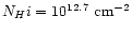 .
Short-dashed and
long-dashed lines represent the
and
Poisson
errors. .
Short-dashed and
long-dashed lines represent the
and
Poisson
errors. |
Figure 12 shows the velocity correlation strength
at
 km s-1.
To obtain sufficient statistics, the analysis was carried out in
three redshift bins: 1.5<z<2.4 (HE 0515-4414,
J2233-606, and HE 2217-2818),
2.5<z<3.1 (HS 1946+7658 and Q0302-003) and
3.5<z<4.0 (Q0000-263).
km s-1.
To obtain sufficient statistics, the analysis was carried out in
three redshift bins: 1.5<z<2.4 (HE 0515-4414,
J2233-606, and HE 2217-2818),
2.5<z<3.1 (HS 1946+7658 and Q0302-003) and
3.5<z<4.0 (Q0000-263).
In our approach
was estimated averaging 1000 numerical
simulations of the observed number of lines, trying to account for
relevant cosmological and observational effects. In particular
a set of lines was randomly generated in the same redshift
interval as the data according to the cosmological distribution
 ,
with
,
with
 (see Sect. 4.2). The
results are not sensitive to the value of
adopted and even a
flat distribution (i.e.
(see Sect. 4.2). The
results are not sensitive to the value of
adopted and even a
flat distribution (i.e.  )
gives values of
)
gives values of  that differ
typically by less than 0.02. Line blanketing of weak lines due to strong
complexes was also accounted for. Lines with too small velocity
splittings, compared with the finite resolution or the intrinsic
blending due to the typical line widths-the so-called
"line-blanketing'' effect (Giallongo et al. 1996), were
excluded in the estimates of
.
that differ
typically by less than 0.02. Line blanketing of weak lines due to strong
complexes was also accounted for. Lines with too small velocity
splittings, compared with the finite resolution or the intrinsic
blending due to the typical line widths-the so-called
"line-blanketing'' effect (Giallongo et al. 1996), were
excluded in the estimates of
.
Clustering is clearly detected at low redshift: at 1.5<z<2.4 in the
100 km s-1 bin, we measure
 for lines with
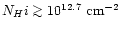 .
There is a hint of increasing amplitude with
increasing column density:
in the same redshift range
.
There is a hint of increasing amplitude with
increasing column density:
in the same redshift range
 for lines with
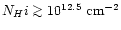 .
The trend is not significant but
agrees with the behavior observed at higher redshifts
(Cristiani et al. 1997; Kim et al. 1997).
Unfortunately the number of lines observed in the interval 1.5<z<2.4does not allow us to extend the analysis to higher column densities,
although groups of strong lines are occasionally evident
(e.g. the range 3230-3270 Å in HE 0515-4414).
.
The trend is not significant but
agrees with the behavior observed at higher redshifts
(Cristiani et al. 1997; Kim et al. 1997).
Unfortunately the number of lines observed in the interval 1.5<z<2.4does not allow us to extend the analysis to higher column densities,
although groups of strong lines are occasionally evident
(e.g. the range 3230-3270 Å in HE 0515-4414).
The amplitude of the correlation at 100 km s-1 decreases
significantly with increasing redshift from
 at
1.5<z<2.4, to
at 2.5<z<3.1 and
at
1.5<z<2.4, to
at 2.5<z<3.1 and
 at
3.5<z<4.0.
at
3.5<z<4.0.
| QSO | Region | Wavelength | |
 |
Comoving size
|
 |
 |
| (Å) | (h-1 Mpc) | ||||||
| HE 0515-4414 | A | 3088-3161 | 1.570 | 0.060 | 61.1 | 5.7 | 0.045 |
| HE 2217-2818 | A | 3504-3579 | 1.913 | 0.062 | 54.3 | 8.4 | 0.012 |
| HE 2217-2818 | B | 3878-3946 | 2.218 | 0.056 | 43.5 | 8.0 | 0.018 |

Voids along the three low-redshift lines of sight were searched for.
For comparison with previous results (Carswell & Rees
1987; Crotts 1987; Ostriker et al. 1988),
we identify a void as a region
without any absorption stronger than
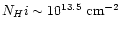 over a comoving size of
at least
over a comoving size of
at least
 Mpc (assuming
 ).
).
Figures 13-14 show the voids
detected in the spectrum of HE 0515-4414 and
HE 2217-2818, respectively. No significant void was found in
the spectrum of J2233-606. The wavelength range used for
searching for voids has been
selected to be redward of the QSO's Ly
emission line and
3000 km s-1 blueward of the QSO's Ly
emission to
avoid the proximity effect. The wavelength range searched for
voids is larger than
that used to study the Ly
forest in other sections.
Table 7 lists the dimensions of the voids,
as well as the probability of finding a void larger than their
comoving size. The probability was calculated assuming a Poisson
distribution of the local forest. In this case, the probability
of finding a void larger than a given size
is
 ,
where
is the line interval in the unit of the local
mean line interval and n is the number of lines with
,
where
is the line interval in the unit of the local
mean line interval and n is the number of lines with
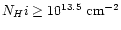 (Ostriker et al. 1988).
The joint probability of finding two voids with a size larger than
(Ostriker et al. 1988).
The joint probability of finding two voids with a size larger than
 Mpc at
  ,
as observed in the spectrum of
HE 2217-2818, is of the order of
,
as observed in the spectrum of
HE 2217-2818, is of the order of
 .
The results correspond very well
to the probability estimates derived from the
simulations described above.
.
The results correspond very well
to the probability estimates derived from the
simulations described above.
There are different ways to produce a void in the forest: a large
fluctuation in the gas density of absorbers, enhanced UV
ionizing radiation from nearby faint QSOs or star-forming galaxies,
feedback processes (including shock heating) from
galaxy formation
(Dobrzycki & Bechtold 1991; Heap et al. 2000;
Theuns et al. 2000a).
We recall here that the void B in the spectrum of HE 2217-2818
corresponds to a region of above-average Doppler parameter (Sect. 4.3.3).
It will be interesting to carry out deep imaging around
HE 2217-2818 to identify QSO candidates and investigate
whether a local ionizing source is responsible for the
 Mpc voids.
![\begin{figure}
\par\includegraphics[width=7.8cm,clip]{H2407F13.eps}\end{figure}](/articles/aa/full/2001/27/aah2407/img370.gif) |
Figure 13: The spectrum of HE 0515-4414 with the void at z = 1.570. See the text for the details. |
Copyright ESO 2001
![\begin{figure}
\includegraphics[width=7.8cm,clip]{H2407F4.eps}\end{figure}](/articles/aa/full/2001/27/aah2407/img129.gif)
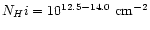
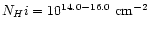


 .
.

![\begin{figure}
\par\includegraphics[width=17.7cm,clip]{H2407F7.eps}\end{figure}](/articles/aa/full/2001/27/aah2407/img227.gif)
 .
Errors are not displayed.
Crosses indicate the data points with
errors less than 25% both
in
.
Errors are not displayed.
Crosses indicate the data points with
errors less than 25% both
in
![\begin{figure}
\par\includegraphics[width=7cm,clip]{H2407F9.eps}\end{figure}](/articles/aa/full/2001/27/aah2407/img323.gif)
![\begin{figure}
\par\includegraphics[width=8.5cm,clip]{H2407F10.eps}\end{figure}](/articles/aa/full/2001/27/aah2407/img330.gif)
 value in the panels indicates the
median b value at the corresponding z for Sample A.
The number in parentheses indicates the
value in the panels indicates the
median b value at the corresponding z for Sample A.
The number in parentheses indicates the
 value from
the Gaussiandistribution.
value from
the Gaussiandistribution.