A&A 494, 287-294 (2009)
DOI: 10.1051/0004-6361:200810660
Markov properties of solar granulation
A. Asensio Ramos
Instituto de Astrofísica de Canarias, 38205 La Laguna, Tenerife, Spain
Received 23 July 2008 / Accepted 25 October 2008
Abstract
Aims. We estimate the minimum length on which solar granulation can be considered to be a Markovian process.
Methods. We measure the variation in the bright difference between two pixels in images of the solar granulation for different distances between the pixels. This scale-dependent data is empirically analyzed to find the minimum scale on which the process can be considered Markovian.
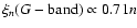
Results. The results suggest that the solar granulation can be considered to be a Markovian process on scales longer than
 km. On longer length scales, solar images can be considered to be a Markovian stochastic process that consists of structures of size
  .
Smaller structures exhibit correlations on many scales simultaneously yet cannot be described by a hierarchical cascade in scales. An analysis of the longitudinal magnetic-flux density indicates that it cannot be a Markov process on any scale.
.
Smaller structures exhibit correlations on many scales simultaneously yet cannot be described by a hierarchical cascade in scales. An analysis of the longitudinal magnetic-flux density indicates that it cannot be a Markov process on any scale.
Conclusions. The results presented in this paper constitute a stringent test for the realism of numerical magneto-hydrodynamical simulations of solar magneto-convection. In future exhaustive analyse, the non-Markovian properties of the magnetic flux density on all analyzed scales might help us to understand the physical mechanism generating the field that we detect in the solar surface.
Key words: Sun: granulation - methods: statistical - Sun: atmosphere
Advances in the study of stochastic processes (Van Kampen 1992) have led to the development of
a powerful set of tools with which to infer important properties about
complex physical systems. An example is the investigation of turbulence (Renner et al. 2001a), where the
energy cascade from large to small scales is responsible for energy transfer in
turbulent fluids (e.g. Frisch 1995). Another case of interest is the analysis of
rough surfaces and interfaces (Jafari et al. 2003; Waechter et al. 2004), where the characterization
of the roughness is of paramount importance for understanding the physical and chemical properties of these
surfaces. Another example is the investigation of the complex time variation of the market
(Renner et al. 2001b).
![\begin{figure}
\par\includegraphics[bb=0 0 504 270,width=8.8cm]{0660f1a.eps}\inc...
...60f1c.eps}\includegraphics[bb=0 0 504 185,width=8.8cm]{0660f1d.eps}
\end{figure}](/articles/aa/full/2009/04/aa10660-08/Timg14.gif) |
Figure 1:
Images used to analyze the Markovian properties of solar granulation.
The images of the upper pane correspond to the G-band
( left) and to Ca II H line,
obtained with the broad-band filters. The images in
the lower panel correspond to images
obtained reconstructed from a scanning with the spectrograph, with the continuum intensity
in the left panel and the magnetic flux density in
the right panel. |
| Open with DEXTER |
The characterization of such complex systems has been carried out historically based on
notions of fractal theory. The idea is to verify the extent to which the cascade from larger
to smaller scales follows a statistical self-similar behavior. In other words, given a physical
quantity x that describes a property of the complex system (for instance, the velocity along a given axis of
a fluid or the height for a surface), we investigate the fluctuation of this
quantity on different scales. In general, it is assumed that the nth statistical moment of the
fluctuation of x (also known as the structure function) fulfills:
 |
(1) |
where r is the considered scale and  is an exponent that depends on n. If
depends
linearly on n, it is said that the complex system is self-affine. In such a case, its properties
are statistically invariant under a scale transformation, and the system is, consequently, self-similar or
fractal. This was suggested by Kolmogorov (1941) for the turbulent cascade in fluid turbulence. If
is non-linear, the complex system is said to be multi-affine, and its properties must be defined
using an infinity of scaling exponents. This is also true for more refined models of turbulence
(Landau & Lifschitz 1987), in which the complex system exhibits what is referred to as
multi-fractal properties. For more details about these models of turbulence, we
refer to the book by Frisch (1995).
is an exponent that depends on n. If
depends
linearly on n, it is said that the complex system is self-affine. In such a case, its properties
are statistically invariant under a scale transformation, and the system is, consequently, self-similar or
fractal. This was suggested by Kolmogorov (1941) for the turbulent cascade in fluid turbulence. If
is non-linear, the complex system is said to be multi-affine, and its properties must be defined
using an infinity of scaling exponents. This is also true for more refined models of turbulence
(Landau & Lifschitz 1987), in which the complex system exhibits what is referred to as
multi-fractal properties. For more details about these models of turbulence, we
refer to the book by Frisch (1995).
The problem with the scaling analysis is that complex systems exhibit scaling properties for a reduced
range of scales. Following this procedure we then obtain only partial information about the
statistical properties of the system. Furthermore, the range of scales under which the system presents
scaling properties cannot be known a priori. For this reason, there has been
increased interest in the statistical description of these complex systems by direct estimation
of the probability distribution functions of the fluctuations on
different scales,
 .
Examples of this direct approach can be found in the literature (e.g. Friedrich et al. 2000; Ghasemi et al. 2006).
.
Examples of this direct approach can be found in the literature (e.g. Friedrich et al. 2000; Ghasemi et al. 2006).
The crucial idea behind the new approach is the idea of identifying the complex system as a stochastic
process in scales (differences of time and/or space) rather than purely in time
or space. This different point of view allows us to obtain information
about the correlation between different scales and analyze how the physical properties are related
at different scales. Furthermore, it allows us to analyze the complex system without assuming regions
of scaling behavior. As we show below, a substantial simplification in the statistical description of
the system occurs if the Markovian property holds. In this case, the statistical properties on
a given scale depend only on what happens on the next scale, and no correlation is found between
other scales. Almost every stochastic process (at least many processes that are important in physics)
can be considered Markovian on scales longer than a given threshold, which is
usually referred to as the Markovian length
(or time, in case a process in time is being
considered). The breaking of the Markovian property
on scales below the threshold can be identified from the
appearance of coherences in the system. For instance,
the motion of a photon in a stellar atmosphere can be considered to be a Markovian process on scales above
its mean free path.
Concerning solar research, Janßen et al. (2003) analyzed the fractal properties of observed
images of small-scale magnetic structures in speckle-reconstructed magnetograms using the
area-perimeter relation. They compared the results with magneto-convection simulations of the
solar surface, and concluded that solar (and simulated) magnetograms are self-similar on a wide
range of scales with a fractal dimension close to 1.4. Stenflo & Holzreuter (2003,2002)
demonstrated that the distribution of magnetic flux density appears to have fat tails (with respect to a
Gaussian distribution) irrespective of the spatial resolution. They demonstrated this self-similarity by
comparing full-disk magnetograms with both MDI magnetograms and data obtained at the
Swedish La Palma Observatory. More recently,
Abramenko (2005) considered the fact that magnetograms in active regions show
several scaling regions and that the structure function must be considered multi-affine.
A multi-fractal approach is then necessary and they found indications of time evolution
in the multi-fractal properties of active regions, which can be associated with its degree
of criticality.
We investigate the scales on which solar granulation can be considered to be a Markovian
process in scale. This sheds some light on the scales involved in the generation
of the granulation pattern. To this end, we investigate large images of solar granulation obtained with
the Hinode satellite.
The data that we analyze consists of two broad-band filter images taken with
the Solar Optical Telescope (SOT, Tsuneta & et al. 2007) aboard Hinode
on 2007 December 10 at 16:20. Additionally, we also analyzed the horizontal variation in
the continuum intensity at 630 nm and the longitudinal magnetic flux density in an observation close to disk center
carried out on 2007 March 10 starting at 11:37 and lasting for almost 3 h
(Lites et al. 2008). The flux density was measured using the Stokes V profile
observed with the SOT/SP in the Fe I doublet at 630 nm and using the weak-field approximation.
We are aware that these measurements may differ from the true magnetic flux density because the fields may
not be in the weak-field regime of the Zeeman effect. However, since we focus
on the horizontal variation in the maps,
small differences in the absolute value of the magnetic flux will not influence
our conclusions significantly. The images are shown in
Fig. 1. The image of the upper left panel is taken with a filter in
the G-band and the image of the upper right panel is taken with a filter in the Ca II
H line. The exposure time of these images is 0.1 s, and were centered on the disk center.
After calculating the power spectrum of the image, we estimate the spatial resolution
of the observations to be 
 (the scale on which the power spectrum is of the same level
as the high frequency noise), a value that appears to be independent of the exact wavelength of the filter
and is similar to the diffraction limit at 630 nm. The lower panel of
Fig. 1 shows
the continuum intensity (left) reconstructed from the slit scanning and the longitudinal
magnetic flux density (right) images. The image
in the G-band is representative of typical granulation with bright regions
corresponding to magnetized regions. The image with the Ca II H filter presents
a clear inverted granulation pattern with bright integranules and dark granules. Furthermore,
bright regions can be seen coinciding with the bright points in the G-band image.
(the scale on which the power spectrum is of the same level
as the high frequency noise), a value that appears to be independent of the exact wavelength of the filter
and is similar to the diffraction limit at 630 nm. The lower panel of
Fig. 1 shows
the continuum intensity (left) reconstructed from the slit scanning and the longitudinal
magnetic flux density (right) images. The image
in the G-band is representative of typical granulation with bright regions
corresponding to magnetized regions. The image with the Ca II H filter presents
a clear inverted granulation pattern with bright integranules and dark granules. Furthermore,
bright regions can be seen coinciding with the bright points in the G-band image.
![\begin{figure}
\par\mbox{\includegraphics[width=8.8cm]{0660f2a.eps}\includegraph...
...th=8.8cm]{0660f2c.eps}\includegraphics[width=8.8cm]{0660f2d.eps} }\end{figure}](/articles/aa/full/2009/04/aa10660-08/Timg20.gif) |
Figure 2:
Structure functions for the four considered images. The order corresponds to that
found in Fig. 1. The length of the data allows to recover the structure
function up to n=6 without much noise. The dotted lines present linear fits to each Sn in the scaling region. |
| Open with DEXTER |
It is important to note that, instead of the magnetic flux density, one could have analyzed
quantities such as B2 that should be more related to the thermodynamical
properties of the plasma. However, at the spatial resolution that can be achieved
presently, the inference of the modulus of the magnetic field vector is, in general, model-dependent.
For this reason, we prefer to focus on the longitudinal magnetic flux density that is more
straightforwardly related to the observables. We propose to analyze
the markovian properties of other magnetic properties in future work.
We investigate the stochastic properties of the intensity increment:
|
hr(x,y) = I(x',y')-I(x,y),
|
(2) |
where I(x,y) is the intensity of the image at pixel (x,y), while
I(x',y') is the value for a pixel located at a distance r (either in the horizontal
or vertical direction). The intensity increment is a measure of the ``roughness''
of the image and describes the significance of
the intensity variation on different scales. We extract series of 106realizations of this quantity on each scale r for the broad-band images
and 105 for the spectropolarimetric data by selecting points (x,y)
in the field of view and verifying that the point (x',y') is inside the image.
We consider various scales in the horizontal direction. However,
we verified that no anisotropy is detected in the
Markovian properties of the intensity increment when the same exercise is carried out
in the vertical direction. One would expect some
anisotropy in regions where the granulation is strongly modified by the presence of
nearby structures, so that the physical processes responsible for the formation of
the solar granulation can differ in different directions. For instance, the modified
granulation pattern produced by the emergence of magnetic flux tubes simulated by
Cheung et al. (2007) should produce anisotropies in the Markovian properties of the granulation
pattern because of the privileged direction introduced by the presence of the flux tube.
Prior to empirically analyzing the statistical properties of the considered images, we investigate
the scaling behavior of the structure functions:
 |
(3) |
which are equivalent to the moments of the brightness fluctuation fields. First of all,
it is important to note that the following analysis depends on the exact functional form of the
fluctuation field, which we chose to be given by Eq. (2).
The results are shown in
Fig. 2, such that each panel is associated with the corresponding
panels of Fig. 1.
They indicate clearly that a scaling region (
 )
is found in all cases on
a subset of the considered values of r. If we choose the smallest scaling range, we find that
the structure function for the G-band case is self-similar on scales below
200 km, while
the value increases to 300 km for the
Ca II H filter. Concerning the red continuum
case, the scaling range is bounded from below around 100 km and from above at
300 km.
Finally, the structure function for the magnetic flux can be considered self-similar only
below 80 km. Note that the structure functions for the magnetic flux are far noisier,
probably due to the lower number of points in the image and significant amount of noise
present because it is reconstructed from spectropolarimetric data.
)
is found in all cases on
a subset of the considered values of r. If we choose the smallest scaling range, we find that
the structure function for the G-band case is self-similar on scales below
200 km, while
the value increases to 300 km for the
Ca II H filter. Concerning the red continuum
case, the scaling range is bounded from below around 100 km and from above at
300 km.
Finally, the structure function for the magnetic flux can be considered self-similar only
below 80 km. Note that the structure functions for the magnetic flux are far noisier,
probably due to the lower number of points in the image and significant amount of noise
present because it is reconstructed from spectropolarimetric data.
The previous results indicate that all cases can be considered correctly to be self-affine because depends linearly on n in the scaling range. Due to the relatively small size of the data series,
the structure functions are only representative for  .
In this range, the following
values are found for the slopes:
.
In this range, the following
values are found for the slopes:
 ,
,
 ,
,
 ,
,
 .
.
![\begin{figure}
\par\mbox{\includegraphics[width=8.8cm]{0660f3a.eps}\includegraph...
...h=8.8cm]{0660f3c.eps}\includegraphics[width=8.8cm]{0660f3d.eps} }
\end{figure}](/articles/aa/full/2009/04/aa10660-08/Timg28.gif) |
Figure 3:
Unconditional pdf p(h,r) for a set of scales indicated in the legend. The values of hr are
normalized to
 calculated for the largest value of r whose value is indicated in each
panel. The panels correspond to the G-band ( upper left panel),
Ca II H ( upper right panel),
continuum at 630 nm ( lower left panel) and magnetic flux
( lower right panel).
calculated for the largest value of r whose value is indicated in each
panel. The panels correspond to the G-band ( upper left panel),
Ca II H ( upper right panel),
continuum at 630 nm ( lower left panel) and magnetic flux
( lower right panel). |
| Open with DEXTER |
![\begin{figure}
\par\mbox{\includegraphics[width=8.3cm]{0660f4a.eps}\includegraph...
...th=8.3cm]{0660f4c.eps}\includegraphics[width=8.3cm]{0660f4d.eps} }\end{figure}](/articles/aa/full/2009/04/aa10660-08/Timg29.gif) |
Figure 4:
Each block of four plots in this figure presents contour plots of the conditional
pdfs
 (solid lines) and
 (dashed lines) to verify the Markovian
character of the brightness fluctuation, together with two cuts at
(dashed lines) to verify the Markovian
character of the brightness fluctuation, together with two cuts at
 .
Each block of four plots corresponds to each image in Fig. 1. For the G-band and
Ca II H data, we have used
r1=395 km while .
Each block of four plots corresponds to each image in Fig. 1. For the G-band and
Ca II H data, we have used
r1=395 km while
 km for the left panel of each block and km for the left panel of each block and
 km
for the right panel of each block. For the spectropolarimetric data (continuum at 630 nm and magnetic flux), these values are
r1=1070 km and km
for the right panel of each block. For the spectropolarimetric data (continuum at 630 nm and magnetic flux), these values are
r1=1070 km and
 km
( left panel) and km
( left panel) and
 km ( right panel). km ( right panel). |
| Open with DEXTER |
We summarize the properties of Markov processes that we use in this paper. All
these properties can be found in any suitable book on stochastic processes (e.g. Van Kampen 1992).
We assume that the variable h(r) defined by Eq. (2) fulfills
a stochastic process in the scale r. To describe the stochastic process completely,
we need to calculate the joint n-scale probability distribution function (PDF)![[*]](/icons/foot_motif.gif)
 ,
which indicates the probability of obtaining the value of the
variable h1 on scale r1, the value h2 on scale r2, and, in general, the value hn on
scale rn. We note that we assume that the scales are ordered following
,
which indicates the probability of obtaining the value of the
variable h1 on scale r1, the value h2 on scale r2, and, in general, the value hn on
scale rn. We note that we assume that the scales are ordered following
 .
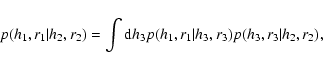
Without losing generality, the joint PDF can be factorized by using the conditional PDFs, as
.
Without losing generality, the joint PDF can be factorized by using the conditional PDFs, as
where
p(hn,rn) is the probability of hn being on scale rn and
p(hm,rm|hn,rn) is the conditional probability, which indicates the probability of
hm being on scale rm provided that hn is found on scale rn. The
quantity
p(hn,rn) is known as the marginal probability distribution function,
which is referred hereafter as PDF (on a given scale). According
to Bayes' theorem, this conditional probability can be written as:
 |
(5) |
Although all the physics of the stochastic problem is contained in the
joint PDF, unfortunately the joint PDF cannot be derived empirically, due to the
enormous amount of data that one would require to complete such an estimation. Consequently, a simplification
is mandatory, and can be created if one considers that the stochastic process can
be classified as Markovian, so that:
 |
(6) |
In other words, the probability of having h1 on scale r1, which in general depends on the complete
history of the process on all scales, does only depend on the value of h2 on scale r2. Consequently,
a Markov process is a process without memory, because the previous history of the process on different scales is
of no relevance for calculating the probability of a future event. This
simplifies Eq. (4) to read:
| |
|
 |
|
| |
|
 |
(7) |
The most straightforward consequence of the stochastic process being Markovian is that it
can be fully described if one knows the conditional
probability distribution function (CPDF)
p(hn-1,rn-1|hn,rn). The empirical determination of the
CPDF is feasible with a relatively reduced amount of data and is the objective of this work.
As a consequence of the relation given by Eq. (6)
any Markovian process fulfills the Chapman-Kolmogorov equation:
 |
(8) |
for any value of r3 such that
r1 < r3 < r2. A usual interpretation of the previous equation
is that the probability of having h1 on scale r1 provided that h2 is found on scale r2 can
be obtained because of the infinite ``paths'' through states on an intermediate scale r3. The
Chapman-Kolmogorov equation is of fundamental importance because it can be formulated
in differential form, which becomes the well-known Kramers-Moyal expansion
(Van Kampen 1992):
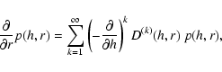 |
(9) |
where
D(k)(h,r) are the Kramers-Moyal coefficients, whose knowledge is sufficient to describe
the Markovian stochastic process completely. Another simplification arises when only
D(1)(h,r) (drift) and
D(2)(h,r) (diffusion) are of importance, and the remaining
coefficients are very close to zero. According to Pawula's theorem (Pawula 1967), this occurs provided
that
 .
In this case, we derive the well-known
Fokker-Planck equation:
.
In this case, we derive the well-known
Fokker-Planck equation:
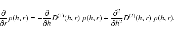 |
(10) |
The coefficients
D(1)(x,r) and
D(2)(x,r) can be estimated empirically from a large set of
data (Friedrich et al. 2000), which allows us to describe fully the statistical properties of the
stochastic process by the solution of the Fokker-Planck equation, directly
obtaining the PDF, p(h,r) or the conditional PDFs,
p(h1,r1|h2,r2).
The scope of this paper is to verify the Markovian properties of solar granulation. The
possibility of using a Fokker-Planck equation to describe the granulation as a
random field on scales will be assesed in a future paper. This would allow us, for instance, to
construct artificially granulation images that have the same statistical properties as the
real ones.
![\begin{figure}
\par\mbox{\includegraphics[width=8.8cm]{0660f5a.eps}\includegraph...
...th=8.8cm]{0660f5c.eps}\includegraphics[width=8.8cm]{0660f5d.eps} }\end{figure}](/articles/aa/full/2009/04/aa10660-08/Timg46.gif) |
Figure 5:
Value of
 for several values of r1 and
  The horizontal
solid line indicates the value
The horizontal
solid line indicates the value
 .
Each panel corresponds to each panel of Fig. 1. .
Each panel corresponds to each panel of Fig. 1. |
| Open with DEXTER |
Figure 3 shows the PDF, p(h,r), on different scales as indicated in the
legend. Due to the difference in pixel size between the broad-band images and
the spectropolarimetric data we note that the length scales at which the magnetic flux and the
continuum at 630 nm are analyzed are a factor 2.5 larger than for the broad-band images.
The brightness difference hr on all scales is normalized by the standard deviation of hr on the largest scale, i.e.,
,
whose respective values
are indicated in each panel of Fig. 3.
The results for the G-band are distributions that are close to Gaussians except in the
extreme tails. On scales larger than the largest shown in Fig. 3, the PDFs overlap.
The bumps around
 and
and
 might be associated with the presence of bright points that induce larger fluctuations than
one would expect without these bright points. This conclusion is reinforced by the fact that
the results for the continuum at 630 nm do not exhibit such bumps. For comparison,
we emphasize that the PDF of fluctuations in pure Gaussian
noise is normal with
might be associated with the presence of bright points that induce larger fluctuations than
one would expect without these bright points. This conclusion is reinforced by the fact that
the results for the continuum at 630 nm do not exhibit such bumps. For comparison,
we emphasize that the PDF of fluctuations in pure Gaussian
noise is normal with
 ,
independent of
scale. The results shown in Fig. 3 indicate that noise is not dominant because the
PDFs vary with scale. Of interest is the fact that the PDFs for the Ca II
H filter present heavy tails that cannot be explained by a Gaussian distribution. This is a consequence
of the appearance of bright and dark points in the image (produced by the presence of strongly
magnetized regions). Furthermore, large variations in the brightness difference can be found on almost all
scales, producing fat tails of exponential type. A similar behavior is found in the flux distribution.
In this case, however, the PDFs differ significantly from Gaussian with tails
that have a Lorentzian shape. The fat tails found for the flux PDF are indicative of
a strongly intermitent process, in which significant fluctuations have an unusually high probability
of occurring compared to that for a Gaussian process. Similar PDFs but for the flux distribution
itself were obtained by Stenflo & Holzreuter (2003,2002), which apparently also exhibited
a Lorentzian shape independent of scale.
,
independent of
scale. The results shown in Fig. 3 indicate that noise is not dominant because the
PDFs vary with scale. Of interest is the fact that the PDFs for the Ca II
H filter present heavy tails that cannot be explained by a Gaussian distribution. This is a consequence
of the appearance of bright and dark points in the image (produced by the presence of strongly
magnetized regions). Furthermore, large variations in the brightness difference can be found on almost all
scales, producing fat tails of exponential type. A similar behavior is found in the flux distribution.
In this case, however, the PDFs differ significantly from Gaussian with tails
that have a Lorentzian shape. The fat tails found for the flux PDF are indicative of
a strongly intermitent process, in which significant fluctuations have an unusually high probability
of occurring compared to that for a Gaussian process. Similar PDFs but for the flux distribution
itself were obtained by Stenflo & Holzreuter (2003,2002), which apparently also exhibited
a Lorentzian shape independent of scale.
Although the images are large, the use of Eq. (6) is insufficient
for estimating the Markovian properties on all scales. However, it is sufficient for testing the
Markovian character on three scales:
| |
|
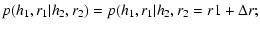 |
|
| |
|
 |
(11) |
where we chose h3=0 and
 for simplicity. In any case, we verified that
the same results were obtained for different values of h3. The previous equality must be verified
for all values of
and h2. Figure 4 presents some examples of the
conditional PDFs
p(h1,r1|h2,r2) and
for simplicity. In any case, we verified that
the same results were obtained for different values of h3. The previous equality must be verified
for all values of
and h2. Figure 4 presents some examples of the
conditional PDFs
p(h1,r1|h2,r2) and
 ,
where the values of r1 and
are given in the caption. The empirical conditional PDFs were
calculated by constructing two-dimensional
histograms. We present cuts along
,
where the values of r1 and
are given in the caption. The empirical conditional PDFs were
calculated by constructing two-dimensional
histograms. We present cuts along
 below each contour plot.
Although not exhaustive, the calculations demonstrate that the processes are not Markovian for the smallest
value of ,
while
p(h1,r1|h2,r2) and
almost overlap for the largest value of .
This only happens for the G-band, Ca II H, and continuum images, and implies
that there is a threshold scale smaller than which the stochastic process generating
the images cannot be considered to be Markovian, while the process is Markovian above this scale.
In contrast,
the calculations for the magnetic flux indicate that, apparently, there is no scale above which the
process can be considered to be Markovian.
below each contour plot.
Although not exhaustive, the calculations demonstrate that the processes are not Markovian for the smallest
value of ,
while
p(h1,r1|h2,r2) and
almost overlap for the largest value of .
This only happens for the G-band, Ca II H, and continuum images, and implies
that there is a threshold scale smaller than which the stochastic process generating
the images cannot be considered to be Markovian, while the process is Markovian above this scale.
In contrast,
the calculations for the magnetic flux indicate that, apparently, there is no scale above which the
process can be considered to be Markovian.
Since a more thorough characterization of the Markovian properties is desired, we applied the
Wilcoxon test (see, e.g. Renner et al. 2001a) that we briefly describe.
We assume that x and y are two stochastic variables with
unknown probability distribution functions p(x) and p'(y), respectively.
By using the two samples
 and
and
 ,
the
Wilcoxon test verifies whether the two
PDFs p(x) and p'(y) are equivalent. In our case, since we wish to verify the validity of
Eq. (11), xi corresponds to samples of the brightness
fluctuation h1 on scale r1 where h2 has been found on scale r2, while yj corresponds
to samples of h1 on scale r1 where h2 and h3 have been found on scales r2 and r3, respectively.
The test sorts the realizations of x and y in ascending order and counts
the number of inversions. In other words, for each value of yj, we count the total number Q of
values xi that fulfill xi < yj. In the case that
p(x)=p'(y), the
quantity Q is distributed
normally about
,
the
Wilcoxon test verifies whether the two
PDFs p(x) and p'(y) are equivalent. In our case, since we wish to verify the validity of
Eq. (11), xi corresponds to samples of the brightness
fluctuation h1 on scale r1 where h2 has been found on scale r2, while yj corresponds
to samples of h1 on scale r1 where h2 and h3 have been found on scales r2 and r3, respectively.
The test sorts the realizations of x and y in ascending order and counts
the number of inversions. In other words, for each value of yj, we count the total number Q of
values xi that fulfill xi < yj. In the case that
p(x)=p'(y), the
quantity Q is distributed
normally about
 with variance
 .
Consequently, the average value of the quantity
.
Consequently, the average value of the quantity
 over h2fulfills
 .
.
Applying the previous test to the brightness fluctuation fields, we obtained the results
shown in Fig. 5. We first focus on our results for the
G-band, Ca II H, and
continuum. The value of
for many values of
r1 and
support the assertion that the process is Markovian above a scale
that is in the range 300-500 km and the Markovian properties are maintained on larger scales.
Above
 and apart from the dispersion produced by the presence
of statistical noise in the determination of
,
all values are distributed about the
value
and apart from the dispersion produced by the presence
of statistical noise in the determination of
,
all values are distributed about the
value
 ,
which implies that the two distributions of
Eq. (11) can be assumed to be the identical. We verified
that the same results for
are obtained when other values of h3 are chosen, which
demonstrates the reliability of the determination of the Markovian scale.
,
which implies that the two distributions of
Eq. (11) can be assumed to be the identical. We verified
that the same results for
are obtained when other values of h3 are chosen, which
demonstrates the reliability of the determination of the Markovian scale.
The previous analysis demonstrates that there are slight differences between the value of
for
different images, with a larger value being measured for the Ca II H filter (
 km) than for
both the G-band and the continuum at 630 nm (
km) than for
both the G-band and the continuum at 630 nm (
 km). Therefore, the images can be considered as
structures of sizes approximately equal to
that are described by a Markovian stochastic process.
Above ,
the brightness fluctuations on a given scale depend only on the next largest scale
(as in a hierarchical cascade) and whatever the nature of the fluctuation
is on a large scale, it does not affect directly
the fluctuations on small scales. A direct consequence of the Markovian character is that
the PDF can be described by the diffusion memoryless Fokker-Planck equation (provided that
)
and can be considered to be a diffusion process on a range of different scales.
Following previous works (e.g. Friedrich et al. 2000),
the Fokker-Planck equation can be reconstructed empirically by estimating the drift and diffusion
coefficients. The numerical solution of the Fokker-Planck equation should allow us to generate
artificial images that have the same statistical properties as the observed ones, although this is
presently ongoing work.
km). Therefore, the images can be considered as
structures of sizes approximately equal to
that are described by a Markovian stochastic process.
Above ,
the brightness fluctuations on a given scale depend only on the next largest scale
(as in a hierarchical cascade) and whatever the nature of the fluctuation
is on a large scale, it does not affect directly
the fluctuations on small scales. A direct consequence of the Markovian character is that
the PDF can be described by the diffusion memoryless Fokker-Planck equation (provided that
)
and can be considered to be a diffusion process on a range of different scales.
Following previous works (e.g. Friedrich et al. 2000),
the Fokker-Planck equation can be reconstructed empirically by estimating the drift and diffusion
coefficients. The numerical solution of the Fokker-Planck equation should allow us to generate
artificial images that have the same statistical properties as the observed ones, although this is
presently ongoing work.
It is interesting to note that the derived
for the
G-band and continuum cases is smaller than the average granular size, defined
to be the FWHM of the autocorrelation function.
The inner properties of structures with sizes smaller than
cannot be described by a Markov
process because of the presence of coherences. As a consequence, their statistical properties cannot
be described using either the Chapman-Kolmogorov or the Kramers-Moyal expansion, so that
the structures must be characterized by determining the joint n-scale probability
distribution function on all scales below .
The results for the magnetic flux are remarkable because they imply that the stochastic process
does not fulfill a Markovian process on any scale (except perhaps on the smallest considered
scale when r1=107 km). We verified that the same behavior for
was found when
larger values of
(i.e. as large as several Mm) are considered. This behavior states that the
probability distribution function of the magnetic flux fluctuations on a given scale depends
on events occurring on all other scale. A more in-depth analysis of this fact could help
us understand the relation between the lack of Markovian character
and the physical mechanism generating the magnetic field
(Asensio Ramos et al. 2009, in preparation).
We have presented an in-depth analysis of the stochastic properties of the difference in the brightness
of two pixels separated by a distance r. The solar telescope onboard Hinode was
used to obtain broad-band filter images. We estimated the
limiting scale above which the stochastic process could be considered to be Markovian. Application
of the Wilcoxon test implied that on scales above 300 km for the G-band and
red continuum images, and above 500 km for Ca II H data, a Markovian behavior is
exhibited. In such a case, the brightness fluctuation on a given scale depends only on events on the
immediate larger scale. We also applied the same analysis to the magnetic flux inferred
from spectropolarimetric observations carried out with SOT/SP onboard Hinode. The results
indicated that the fluctuations in the magnetic flux cannot be considered to be Markovian, so that
the PDF on a given scale depends on what is happening on all other scales.
The completely different behaviors of the brightness and magnetic flux
imply that this should also be found for any successful
numerical MHD simulation of solar
magneto-convection (Stein & Nordlund 2006; Vögler et al. 2005). Since this test analyzes how the physical
quantities change on different scales and how they are related, we can investigate if the
sizes of the computational boxes are of the correct size for capturing the true behavior of
the turbulent convection and the ensuing motion of the magnetic field. The present MHD simulations
are carried out in quite small computational boxes (of the order of
 Mm2), and
it remains to be determined the extent to which the analysis that we have presented here
can be applied to far smaller fields-of-view.
Mm2), and
it remains to be determined the extent to which the analysis that we have presented here
can be applied to far smaller fields-of-view.
Acknowledgements
I thank H. Frisch and J. Trujillo Bueno for useful comments on the manuscript.
This research has been funded by the Spanish Ministerio de Educación y Ciencia
through project AYA2007-63881.
- Abramenko,
V. I. 2005, Sol. Phys., 228, 29 [NASA ADS] [CrossRef]
(In the text)
- Cheung,
M. C. M., Schüssler, M., & Moreno-Insertis, F.
2007, A&A, 467, 703 [NASA ADS] [CrossRef] [EDP Sciences]
(In the text)
- Friedrich,
R., J., P., & Renner, C. 2000, , 84, 5224
- Frisch, U. 1995,
Turbulence (Cambridge University Press)
(In the text)
- Ghasemi, F.,
Bahraminasab, A., Sadegh Movahed, M., et al. 2006, J. Stat.
Mech., 11008
-
Jafari, G. R., Fazeli, S. M., Ghasemi, F., et al.
2003, Phys. Rev. Lett., 91, 226101 [NASA ADS] [CrossRef]
- Janßen, K.,
Vögler, A., & Kneer, F. 2003, A&A, 409, 1127 [NASA ADS] [CrossRef] [EDP Sciences]
(In the text)
- Kolmogorov,
A. N. 1941, Dokl. Akad. Nauk. SSSR, 30, 301 [NASA ADS]
(In the text)
- Lites, B. W.,
Kubo, M., Socas-Navarro, H., et al. 2008, ApJ, 672, 1237 [NASA ADS] [CrossRef]
(In the text)
- Pawula, R. F.
1967, Phys. Rev., 162, 186 [NASA ADS] [CrossRef]
(In the text)
- Renner, C., J., P.,
& Friedrich, R. 2001a, J. Fluid Mech., 433, 383 [NASA ADS]
(In the text)
-
Renner, C., Peinke, J., & Friedrich, R. 2001b, Physica A, 298,
499 [NASA ADS] [CrossRef]
(In the text)
- Stein, R. F.,
& Nordlund, Å. 2006, ApJ, 642, 1246 [NASA ADS] [CrossRef]
- Stenflo, J. O., &
Holzreuter, R. 2002, in SOLMAG 2002. Proceedings of the Magnetic
Coupling of the Solar Atmosphere Euroconference, ed.
H. Sawaya-Lacoste, ESA SP, 505, 101
- Stenflo, J. O., &
Holzreuter, R. 2003, in Current Theoretical Models and Future High
Resolution Solar Observations: Preparing for ATST, ed. A. A.
Pevtsov, & H. Uitenbroek, ASP Conf. Ser., 286, 169
-
Tsuneta, S., et al. 2007, Sol. Phys., submitted
(In the text)
- Vögler, A.,
Shelyag, S., Schüssler, M., et al. 2005, A&A, 429,
335 [NASA ADS] [CrossRef] [EDP Sciences]
-
Van Kampen, N. G. 1992, Stochastic Processes in Physics
and Chemistry (North Holland)
(In the text)
-
Waechter, M. F. R., Schimmel, T., Wendt, U., & Peinke, J. 2004,
Eur. J. Phys. B, 41, 259 [NASA ADS] [CrossRef]
Copyright ESO 2009
![\begin{figure}
\par\includegraphics[bb=0 0 504 270,width=8.8cm]{0660f1a.eps}\inc...
...60f1c.eps}\includegraphics[bb=0 0 504 185,width=8.8cm]{0660f1d.eps}
\end{figure}](/articles/aa/full/2009/04/aa10660-08/img14.gif)
![\begin{figure}
\par\mbox{\includegraphics[width=8.8cm]{0660f2a.eps}\includegraph...
...th=8.8cm]{0660f2c.eps}\includegraphics[width=8.8cm]{0660f2d.eps} }\end{figure}](/articles/aa/full/2009/04/aa10660-08/img20.gif)
![\begin{figure}
\par\mbox{\includegraphics[width=8.8cm]{0660f3a.eps}\includegraph...
...h=8.8cm]{0660f3c.eps}\includegraphics[width=8.8cm]{0660f3d.eps} }
\end{figure}](/articles/aa/full/2009/04/aa10660-08/img28.gif)
![\begin{figure}
\par\mbox{\includegraphics[width=8.3cm]{0660f4a.eps}\includegraph...
...th=8.3cm]{0660f4c.eps}\includegraphics[width=8.3cm]{0660f4d.eps} }\end{figure}](/articles/aa/full/2009/04/aa10660-08/img29.gif)
![\begin{figure}
\par\mbox{\includegraphics[width=8.8cm]{0660f5a.eps}\includegraph...
...th=8.8cm]{0660f5c.eps}\includegraphics[width=8.8cm]{0660f5d.eps} }\end{figure}](/articles/aa/full/2009/04/aa10660-08/img46.gif)