A&A 493, 697-710 (2009)
DOI: 10.1051/0004-6361:200809853

Breit-Pauli R-matrix calculation for fine structure effective collision strengths from electron impact excitation of Mg IX

C. E. Hudson

School of Mathematics and Physics, The Queens University of Belfast, Belfast BT7 1NN, Northern Ireland, UK

Received 26 March 2008 / Accepted 20 October 2008

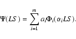
Abstract
Context. Electron impact excitation collision strengths are required for analysing and interpreting stellar observations.
Aims. This calculation aims to provide fine-structure effective collision strengths for the Mg IX ion using a method that includes contributions from resonances.
Methods. A 26-state Breit-Pauli R-matrix calculation has been performed. The target states are represented by configuration interaction wavefunctions and consist of the 26 lowest ${\it LS}$ states, having configurations 2s², 2s2p, 2p², 2s3s, 2s3p, 2s3d, 2p3s, 2p3p, and 2p3d. These target states give rise to 46 fine structure levels and 1035 possible transitions. The effective collision strengths are calculated by averaging the electron collision strengths over a Maxwellian distribution of electron velocities.
Results. The non-zero effective collision strengths for transitions between the fine structure levels are given for electron temperatures ($T_{\rm e}$) in the range $\log_{10} T_{\rm e}$(K) = 3.0-7.0. Values for selected transitions are given in this paper and links provided to the entire data set.

Key words: atomic processes - line: formation - methods: analytical

1 Introduction

Beryllium-like ions are have been detected in a wide variety of plasmas, e.g. the solar transition region, planetary nebulae, active galactic nuclei and laboratory plasmas. To analyse and interpret the emission lines observed, atomic data in the form of effective collision strengths are needed and the data for specific lines can be used as plasma diagnostics for quantities such as electron temperature, density and abundance.

An example of some lines which have been used as diagnostics, is that of Wilhelm et al. (1998) who make use of the Mg IX lines at 706 and 750 Å  pertinent to both the electron density and electron temperature of polar coronal holes. These lines correspond to the 2s^2 1S₀-2s2p ³P $^{\rm o}_1$ and 2s2p ¹P $^{\rm o}_1$-2p^2 1D₂ transitions.

Recent observations of Mg IX lines include: Bauer et al. (2007) who have observed strong lines of Mg IX in the diffuse X-ray emission in the halo and disc of starburst galaxy NGC 253. Ness et al. (2005) find lines in the X-ray range at 72.3 and 77.7 Å corresponding to 2s2p¹P₁-2s3d¹D₂ and 2s2p ¹P₁-2s3s ¹S₀ observed by the LETGS instrument on ${\it Chandra}$. In the EUV range Maltby et al. (1998) observed the 2s^2 1S₀-2s2p ¹P₁ line at 368 Å with the Coronal Diagnostic Spectrometer (CDS) on SOHO.

Currently in the CHIANTI database (Landi et al. 2006; Dere et al. 1997) there are 188 effective collision strengths recorded for this ion. A total of 46 fine structure levels are noted and for the 45 transitions between levels 1-10, the effective collision strengths are values from Keenan et al. (1986) which have been interpolated from R-matrix calculations for other ions of the same isoelectronic sequence, namely C II, Ne VII and Si XI. These calculations (Berrington et al. 1985,1981) determine results in LS-coupling and involve 6 LS target states. The remaining 143 transitions in CHIANTI are between initial levels 1-5 and final levels 11-46 and are from a Distorted Wave evaluation of Sampson et al. (1984).

However a more recent Distorted-Wave calculation has been performed by Bhatia & Landi (2007) involving 53 LS terms which give rise to 92 fine structure levels. The calculation is carried out in ${\it LS}$-coupling and then the JAJOM transformation of Saraph (1978), with recent modifications by Saraph & Eissner (to be published) was applied to generate the intermediate coupling results. The collision strengths were obtained at seven energies for transitions within the three lowest ${\it LS}$ configurations (2s², 2s2p and 2p²), which correspond to the first 10 fine structure transitions. Values were also given at five energies for transitions between the first five fine structure levels to final levels beyond the three lowest ${\it LS}$ configurations.

In such calculations, however, none of the resonant structure is obtained in the collision strength, and these resonances can significantly enhance the Maxwellian averaged effective collision strengths. To date, no close-coupling calculations have been performed for this ion. Therefore to provide accurate fine structure collisional data for this ion using a method which includes resonances, a sophisticated Breit-Pauli R-matrix calculation has been carried out with 26 LS target states which give rise to 46 j-levels, and a total of 1035 possible fine-structure transitions. Some of these values are presented in this paper, with the remainder being available through the author's website as well as being tabulated at the CDS website.

Table 1: Orbital parameters (c, I, $\zeta$) of the radial wavefunctions.

2 Calculation details

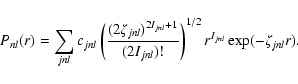
Configuration interaction wavefunctions for the 26 LS target states used in this calculation were constructed using the CIV3 code of Hibbert (1975). Each target-state wavefunction $\Psi$ is represented by a linear combination of single-configuration functions $\Phi_i$, each of which has the same total $LS\pi$ symmetry as the target-state

$$\Psi(LS) = \sum_{i=1}^{m} a_i \Phi_i (\alpha_i LS) .$$ (1)

The $\Phi_i$ in (1) are constructed from a set of one-electron orbitals. The $\alpha_i$ represent the coupling of the angular momenta associated with these one-electron spin orbitals to form the total L and S. The mixing coefficients a_i are determined by the CIV3 code and are eigenvector components of the Hamiltonian matrix having particular LS$\pi$ symmetry. The Hamiltonian matrix elements are defined as

$$H_{ij} = \langle \Phi_i \mid H \mid \Phi_j \rangle$$ (2)

where H denotes the Hamiltonian operator. The one-electron orbitals used to construct the $\Phi_i$ each consist of a radial function, a spherical harmonic and a spin function:

$$u_{nl{m_l}{m_s}}(\vec{r},\sigma) = \frac{1}{r} P_{nl}(r) Y_l^{m_l}(\theta, \phi) \chi_{m_s}(\sigma).$$ (3)

These orbitals are chosen to be analytic, with the radial part being expressed as a sum of normalised Slater-type orbitals:

$$P_{nl}(r) = \sum_{jnl} c_{jnl} \left( \frac{(2\zeta_{jnl})^{... ...{(2I_{jnl})!} \right)^{1/2} r^{I_{jnl}} \exp(- \zeta_{jnl} r).$$ (4)

In this expression, for each orbital, the powers of r (I_jnl) are kept fixed and the coefficients c_jnl and exponents $\zeta_{jnl}$ are treated as variational parameters which are optimised by the CIV3 code. For this calculation the lowest 26 LS states are included as the target states.

In describing these target states ($\Psi$) eight one-electron orbitals were employed, including six real orbitals - 1s, 2s, 2p, 3s, 3p, 3d and to these two pseudo-orbitals were added - a $\overline{4{\rm s}}$ and $\overline{4{\rm p}}$ orbitals as correctors. The orbitals were optimised in the following way: for the 1s and 2s orbitals the values from Fleming et al. (1996) were re-optimised on the average energy of the 1s²2s² and 1s²2p^2 1S states with one of the I_jnl terms being dropped in the expansion for the 2s orbital (see Eq. (4)); for the 2p orbital the parameters determined by Fleming et al. (1996) were used; the 3s, 3p and 3p orbitals were optimised on the average energy of the 2s2p, 2s3p, 2p3s and 2p3d ¹P$^{\rm o}$ levels; the $\overline{4{\rm s}}$ was optimised on the energy of the 2s^2 1S using the four configurations - 2s², 2p², 2s3s, 2s $\overline{4{\rm s}}$ and the $\overline{4{\rm p}}$ orbital was optimised on the energy of the 2p^2 3P using three configurations - 2p², 2p3p, 2p $\overline{4{\rm p}}$. The resulting orbital parameters are shown in Table 1.

The orbitals from Table 1 were used to build a set of single-configuration functions ($\Phi_i$), which were generated by a two electron replacement on the 1s²2s² basis configuration, keeping at least one electron in the 1s shell. Using the 12 symmetries involved in the target state set, this generation leads to a total of 260 configurations - 29 $\times$ ¹S, 13 $\times$ ¹P, 25 $\times$ ¹D, 26 $\times$ ³S, 24 $\times$ ³P, 26 $\times$ ³D, 33 $\times$ ¹P$^{\rm o}$, 9 $\times$ ¹D$^{\rm o}$, 9 $\times$ ¹F$^{\rm o}$, 42 $\times$ ³P$^{\rm o}$, 12 $\times$ ³D$^{\rm o}$ and 12 $\times~^3$F$^{\rm o}$.

Wavefunctions ($\Psi$) for the 26 Mg IX target states are constructed as linear combinations of the single-configuration functions ($\Phi_i$) according to Eq. (1). In Table 2 the target state energies calculated from these wavefunctions are given. Table 2 compares the calculated LS target state energies in Rydbergs (1 Rydberg = 2.17987  $\times 10^{-18}$ J) relative to the 1s²2s^2 1S ground state with values from NIST and those of Bhatia & Landi (2007). The NIST database is available at http://www.physics.nist.gov/PhysRefData and the data for this ion is attributed to Artru (1977), Boiko et al. (1978), Edlen (1979), Fawcett (1970), Hoory et al. (1970), Ridgely & Burton (1972) and Söderqvist (1944). Good agreement is observed between the NIST values and those from the current calculation using the CIV3 structure code, with the current values differing on average by 0.0346 Rydbergs. The calculation of Bhatia & Landi (2007) achieves better agreement with the NIST differing on average by 0.0264 Rydbergs. The configuration set used in the current calculation is quite small in comparison with the calculation of Bhatia & Landi (2007) (this was due to larger sets giving rise to greater numbers of coupled channels in the scattering part of the calculation which on the computer facilities used could not be accommodated). However, for the size of the calculation performed the representation obtained is reasonably good.

As an additional check on the quality of the wavefunctions for the target states, the oscillator strengths produced using the wavefunctions are examined. Oscillator strengths for the allowed transitions between the 26 LS target states are given in Table 3. For the transitions noted in Table 3, there is reasonable agreement between the length and velocity forms ($f_{\rm l}$ and $f_{\rm v}$). Bhatia & Landi (2007) also give oscillator strengths for these transitions and are given in Table 3 (the gf values of Bhatia & Landi (2007) having been converted into f-values). The agreement of the current $f_{\rm l}$ values with the oscillator strengths of Bhatia & Landi (2007) is on the whole quite good - of the 66 non-zero values of Bhatia & Landi (2007), we find that 39 of the current $f_{\rm l}$ values lie within 10 per cent of Bhatia & Landi (2007) (21 are within 5 per cent and 50 within 20 per cent). The largest difference seen is a factor of 2 for transition 12-25 i.e. 2s3d³D-2p3d¹F$^{\rm o}$.

Using these wavefunctions for the Mg IX target ion, the electron-ion collision problem was investigated using the Breit-Pauli R-matrix method (Scott & Burke 1980), employing the RMATRX1 codes of Berrington et al. (Berrington et al. 1987). The version of the codes used here are the serial version available at http://amdpp.phys.strath.ac.uk/tamoc/code.html. The R-matrix radius was calculated to be 4.8 atomic units and for each orbital angular momentum, 20 orthogonalised continuum orbitals were included, ensuring that a converged collision strength was obtained up to an incident electron energy of $\sim$70 Rydbergs.

The (N+1)-electron bound configurations, which are included in the expansion of the (N+1)-electron collision wavefunction to describe the situation when the scattering electron comes close into the target ion were obtained by systematically adding one electron to the N-electron configurations used in the description of the target Mg IX ion.

The current 26 LS state calculation was carried out for all contributing partial waves with $L\leq12$. The mass-correction, Darwin and spin-orbit terms are switched on in the Hamiltonian to produce results in intermediate-coupling. Within the Breit-Pauli framework this gives rise to a 46 fine structure level problem for partial waves up to 2J=27, for both even and odd parity. For optically forbidden transitions, this is sufficient to obtain converged results. However, for optically allowed transitions, additional partial waves or a top-up procedure is required to account for the contribution from these higher partial waves. Therefore to account for partial wave contributions from values of $2J \geq 27$, the partial waves have been topped-up.

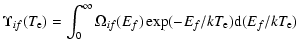
Effective collision strengths $\Upsilon_{if}$ for a particular electron temperature $T_{\rm e}$ were obtained by averaging the electron collision strengths  $\Omega_{if}$ over a Maxwellian distribution of velocities, so that

 

$$\Upsilon_{if}(T_{\rm e})=\int_{0}^{\infty}\Omega_{if}(E_{f}) \exp(-E_{f}/kT_{\rm e}){\rm d}(E_f/kT_{\rm e})$$ (5)

where E_f is the final free electron energy after excitation and k is Boltzmann's constant.

Table 2: Energy levels in Rydbergs for the LS target states included in the calculation, relative to the Mg IX 2s^2 1S ground state.

Table 3: Oscillator strengths for the allowed transitions between the 26 LS target states included in the present calculation. Values are given for the length and velocity forms of the oscillator strength ($f_{\rm l}$ and $f_{\rm v}$). Values from the work of Bhatia & Landi (2007) [B&L] are also noted. (See Table 2 for explanation of labels.)

3 Results and discussion

The collision strengths calculated in this work have been evaluated for a fine mesh of incident impact energies, at energy intervals of 0.0005 Rydbergs ($\sim$ $1.8\times 10^{-6}$ in z-scaled Rydbergs) across the energy range from threshold up to the energy of the last target state considered. This ensured that the autoionizing resonances which converge to the target state thresholds were fully delineated.

Those resonances located at energies lower than the highest target threshold, i.e. 2p3d¹P$^{\rm o}$ at $\sim$16.8 Ryd, are physically meaningful; however at higher energies pseudo-resonances appear. These arise from the inclusion of pseudo-orbitals in the wavefunction expansion (Burke et al. 1981). At higher temperatures the high-impact energy region is much more important and so it is necessary to properly average over the pseudo-resonances to prevent distortion of the correct results in the calculation of the effective collision strengths. Thus above the last target state energy, a coarser mesh of energies is used ($\sim$ $2.5\times 10^{-3}$ in z-scaled Rydbergs). Much of the detail is filtered out and any very large pseudo-resonances are removed, so that in essence a ``background'' level is retained in this region.

Table 4: Fine structure energy levels (in Rydbergs) for the current calculation and the work of Bhatia & Landi (2007), along with the observed values from NIST.

The inclusion of the 26 LS target states leads to 46 J-levels (see Table 4) and a total of 1035 transitions. The fine-structure energies obtained for these J-levels are also shown in Table 4 and are compared to values from Bhatia & Landi (2007) and those from NIST. The current work agrees well with with both the NIST values and the calculation of Bhatia & Landi (2007), with the energies determined by this calculation being within 4% of the NIST values and within 3% of the Bhatia values.

In Figs. 1-5 the collision strengths for the transitions between the first 10 fine structure levels are given. These levels correspond to the 2s² and 2s2p configurations. To show the detail obtained for the resonances the collision strengths are only plotted up to 20 Ryd. Also displayed on these graphs are the values from the Distorted Wave calculation of Bhatia & Landi (2007). For most transitions, excellent agreement is observed between the background levels, but as can be seen, the Distorted Wave calculation does not obtain the resonance structures which can significantly enhance the effective collision strengths. The values of Bhatia & Landi (2007) depart significantly from the current work for transition 1-5 in the resonance region, although at higher energy values they once again agree.

The work of Keenan et al. (1986) provides maxwellian averaged effective collision strengths (see Eq. (5)) with which comparison is made in Figs. 6-8. These values are interpolated data from R-matrix calculations of (Berrington et al. 1985,1981) for C II, Ne VII and Si XI. On Figs. 6-8 the fine structure transitions have been grouped in the same fashion as they were displayed in Keenan et al. (1986), such that transitions between singlet and triplet levels are considered together. Therefore in these cases, the fine structure transitions involved have been summed over. The graphs in Figs. 6-8 carry labels which correspond to the labelling used by Keenan et al. in their paper. These are noted in Table 5 under ``Keenan Labels'' and the transitions to which they correspond using the indices in Table 4 are noted in the column ``Transitions involved''.

As can be seen from Figs. 6-8, for the current calculation, most of the transitions have experienced an enhancement towards high temperatures when compared to the data of Keenan et al. (1986). This is due to the fact that the data of Berrington et al. (1985,1981) which was interpolated to produce these values was gained from calculations which involved the lowest 6 LS terms as target states. Using Table 2 this means that the last target threshold was at an energy of $\sim$4.6 Ryd and so any resonant structure beyond this would not be included. However, from the collision strengths displayed in Figs. 1-5, it is clear that there is considerable structure beyond this point which can contribute to the Maxwellian averaged effective collision strengths.

There are a few transitions where the values of Keenan et al. are higher than the current values, for example in ``keenan transition 7'' in Fig. 6. This could be due to a finer meshsize being employed in the current work and so perhaps some broader resonances are better resolved here, or perhaps an interpolation technique was not adequate for producing data for this ion. ``Keenan transition 28'' is the only one which is vastly disturbing. This corresponds to transitions 6-10, 7-10 and 8-10 in the current work, i.e. 2p^2 3P (J=0, 1, 2)-2p^2 1S, which have been summed over in order to compare with the Keenan et al. (1986) value. The effective collision strength of Keenan et al. (1986) has values in the range 3.27-3.31 whilst the current work peaks at $\sim$0.1. The collision strengths for the transitions involved agree well with values from the Distorted Wave calculation of Bhatia & Landi (2007) and comparing the collision strengths for transitions 6-10, 7-10 and 8-10 with transitions 6-9, 7-9 and 8-9 (see Figs. 4 and 5), each is certainly smaller in magnitude (i.e. comparing 6-10 with 6-9 etc.). Therefore one would expect the effective collision strengths for transitions 6-10, 7-10 and 8-10 to be smaller than those of transitions 6-9, 7-9 and 8-9 and hence their summed values, meaning that ``keenan transition 28'' should be smaller than ``keenan transition 27''. Thus it is suspected that the Keenan et al. (1986) data is in error for this transition.

In the text Table 5: Labels for effective collision strengths shown in Figs. 6-8.

	Figure 1: Collision strengths as a function electron impact energy in Rydbergs (see Table 4 for explanation of labels). Solid line is the Current R-matrix calculation and the circles are values from the work of Bhatia & Landi (2007).
Open with DEXTER

	Figure 2: Collision strengths as a function electron impact energy in Rydbergs (see Table 4 for explanation of labels). Solid line is the Current R-matrix calculation and the circles are values from the work of Bhatia & Landi (2007).
Open with DEXTER

	Figure 3: Collision strengths as a function electron impact energy in Rydbergs (see Table 4 for explanation of labels). Solid line is the Current R-matrix calculation and the circles are values from the work of Bhatia & Landi (2007).
Open with DEXTER

	Figure 4: Collision strengths as a function electron impact energy in Rydbergs (see Table 4 for explanation of labels). Solid line is the Current R-matrix calculation and the circles are values from the work of Bhatia & Landi (2007).
Open with DEXTER

	Figure 5: Collision strengths as a function electron impact energy in Rydbergs (see Table 4 for explanation of labels). Solid line is the Current R-matrix calculation and the circles are values from the work of Bhatia & Landi (2007).
Open with DEXTER

	Figure 6: Transitions 1-10: effective collision strengths as a function log electron temperature (see Table 5 for explanation of labels). Solid line is the Current R-matrix calculation and the dashed line gives the extrapolated values from Keenan et al. (1986).
Open with DEXTER

	Figure 7: Transitions 11-20: effective collision strengths as a function log electron temperature (see Table 5 for explanation of labels). Solid line is the Current R-matrix calculation and the dashed line gives the extrapolated values from Keenan et al. (1986).
Open with DEXTER

	Figure 8: Transitions 21-29: effective collision strengths as a function log electron temperature (see Table 5 for explanation of labels). Solid line is the Current R-matrix calculation and the dashed line gives the extrapolated values from Keenan et al. (1986).
Open with DEXTER

There is excellent agreement between the Keenan et al. (1986) values and the current work for ``Keenan'' transitions 2, 11, 13, 14, 15, 17, 18, 22 and 23. These transitions are allowed in terms of L,S,J and $\pi$ changes.

Table 6, available at CDS, gives the non-zero fine structure effective collision strength data for the 1035 transitions produced in this calculation and contains the following information: Col. 1 lists the transition index noted as i-j (initial-final level) where the levels are given in the accompanying table and correspond to those in Table 4. For example, 2-5 denotes the transition 2s2p ³P $^{\rm o}_0$-2s2p ¹P $^{\rm o}_1$. The remaining columns list the effective collision strengths for each transition at logarithmic electron temperatures $\log_{10} T_{\rm e}$(K) = 3.0-7.0 in steps of 0.2 dex.

4 Conclusions

Effective collision strengths for forbidden and allowed transitions in the electron impact excitation of the Mg IX ion have been calculated. The atomic data are evaluated for the electron temperature range $\log_{10} T_{\rm e}$(K) = 3.0-7.0 and for transitions among the lowest 26 LS states of Mg IX, corresponding to 46 fine structure levels and 1035 individual fine structure transitions. Whilst the overall accuracy is difficult to assess, we expect the current data to have an accuracy of 10%. These calculations provide the first close-coupling evaluations of collision strengths for this ion. Differences exist between the current values and effective collision strengths from previous evaluations.

The effective collision strengths are available at the CDS or alternatively the collision strength and effective collision strength data over the temperature range $\log_{10} T_{\rm e}$(K) = 3.0-7.0 (in steps of 0.1 dex) are available, by contacting the author or via the website http://www.am.qub.ac.uk/apa/data.

Acknowledgements

This work has been supported by PPARC, under the auspices of a Rolling Grant.

References

• Artru, M. C. 1977, unpublished material (In the text)
• Bauer, M., Pietsch, W., Trinchieri, G., et al. 2007, A&A, 467, 979 [NASA ADS] [CrossRef] [EDP Sciences] (In the text)
• Berrington, K. A., Burke, P. G., Dufton, P. L., & Kingston, A. E. 1981, ADNDT, 26, 1 [NASA ADS] [CrossRef]
• Berrington, K. A., Burke, P. G., Dufton, P. L., & Kingston, A. E. 1985, ADNDT, 33, 195 [CrossRef]
• Berrington, K. A., Burke, P. G., Butler, K., et al. 1987, J. Phys. B, 20, 637 [CrossRef] (In the text)
• Bhatia, A. K., & Landi, E. 2007, ADNDT, 93, 742 [NASA ADS] [CrossRef] (In the text)
• Boiko, V. A., Chugunov, A. Y., Ivanov, T. G., et al. 1978, MNRAS, 185, 305 [NASA ADS] (In the text)
• Burke, P., Sukamar, C., & Berrington, K. A. 1981, J. Phys. B, 14, 289 [NASA ADS] [CrossRef] (In the text)
• Dere, K. P., Landi, E., Mason, H. E., Monsignori, B. C., & Young, P. R. 1997, A&AS, 125, 149 [CrossRef] [EDP Sciences]
• Edlen, B. 1979, Phys. Scr., 20, 129 [NASA ADS] [CrossRef] (In the text)
• Fawcett, B. C. 1970, J. Phys. B, 3, 1152 [NASA ADS] [CrossRef] (In the text)
• Fleming, J., Vaeck, N., Hibbert, A., Bell, K. L., & Godefroid, M. R. 1996, Phys. Scr., 53, 446 [NASA ADS] [CrossRef] (In the text)
• Hibbert, A. 1975, Comput. Phys. Comm., 9, 141 [CrossRef] (In the text)
• Hoory, S., Feldman, U., Goldman, S., Behring, W., & Cohen, L. 1970, J. Opt. Soc. Am., 60, 1449 [NASA ADS] [CrossRef] (In the text)
• Keenan, K. P., Berrington, K. A., Burke, P. G., Dufton, P. L., & Kinston, A. E. 1986, Phys. Scr., 34, 216 [NASA ADS] [CrossRef] (In the text)
• Landi, E., Del Zanna, G., Young, P. R., et al. 2006, ApJS, 162, 261 [NASA ADS] [CrossRef]
• Maltby, P., Brynildsen, N., Brekke, P., et al. 1998, ApJ, 2, L117 [NASA ADS] (In the text)
• Ness, J. U., Starrfield, S., Jordan, C., Krautter, J., & Schmitt, J. H. M. M. 2005, MNRAS, 364, 1015 [NASA ADS] [CrossRef] (In the text)
• Ridgely, A., & Burton, W. M. 1972, Sol. Phys., 27, 280 [NASA ADS] [CrossRef] (In the text)
• Sampson, D. H. J. G. S., & Clark, R. E. H. 1984, ADNDT, 30, 125 [NASA ADS] [CrossRef] (In the text)
• Saraph, H. E. 1978, Comput. Phys. Comm., 15, 247 [NASA ADS] [CrossRef] (In the text)
• Saraph, H. E., & Eissner, W., Comput. Phys. Comm., to be published (In the text)
• Scott, N. S., & Burke, P. G. 1980, J. Phys. B, 13, 4299 [NASA ADS] [CrossRef] (In the text)
• Söderqvist, J. 1944, Ark. Mat., Aston. Fys., 30, 1 (In the text)
• Wilhelm, K., Marsch, E., Dwivedi, B. N., et al. 1998, ApJ, 500, 1023 [NASA ADS] [CrossRef] (In the text)