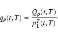
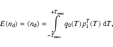
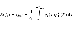
and the correlation time
  as free parameters and investigate their influence on dust formation.
A&A 491, 643-662 (2008)
DOI: 10.1051/0004-6361:20079243
U. Dirks - V. Schirrmacher - E. Sedlmayr
Zentrum für Astronomie und Astrophysik (ZAA), TU Berlin, Hardenbergstr. 36, 10623 Berlin, Germany
Received 13 December 2007 / Accepted 9 July 2008
Abstract
Context. Dust formation, i.e. the condensation of solid particles from a gas phase, occurs in astrophysical environments that are sufficiently cool and offer a sufficiently high density of condensable species. Since many astrophysical systems in which dust forms have turbulent features and the dust formation rates depend significantly on temperature, we investigate the influence of temperature fluctuations on dust condensation in dust-driven AGB winds.
Aims. We present an approach for the time-dependent stochastic description of astrophysical dust formation and apply this in developing a fast algorithm, which is well suited for implementation into numerical models of dynamical AGB winds. The influence of the fluctuations on the dynamical structure is then investigated for a large sample of wind parameters.
Methods. We employ a mathematical method, which describes the dust formation under the influence of random temperature fluctuations as a stochastic process. A system of Fokker-Planck equations for the one-point distribution function of the conjoint temporal development of temperature and dust results. Gas-box studies of this system have led us to a simplified microturbulent description for the implementation into time-dependent numerical wind models.
Results. A method for the investigation of temperature fluctuations on dust formation is presented, which can be adapted to a variety of astrophysical situations. For dust-driven AGB winds, a microturbulent description turns out to be admissible. In AGB winds, rms-temperature fluctuations of 20-60 K can result in increased mass loss rates of 10-30% depending on the details of the physical model assumptions.
Conclusions. The presented method for the treatment of temperature fluctuations with respect to dust formation has been succesfully applied to dynamical AGB winds. We suggest how to apply the method to other astrophysical systems. The influence of the fluctuations on the dynamics of dust-driven AGB winds is remarkable, but not overwhelming.
Key words: turbulence - stars: mass-loss - stars: AGB and post-AGB - stars: winds, outflows - methods: statistical
Dust is an ubiquitous phenomenon in our Galaxy. It is an effective absorber of radiation at short wavelengths and re-emits thermal IR-radiation. Due to this strong interaction between dust and radiation fields, astrophysical situations in which dust formation occurs, often show highly non-linear behaviour in the sense that not only the energy balance of the systems often switches between a dust-free and a dust-enshrouded situation, but also the momentum balance is affected severely by the radiation pressure onto the absorbing dust, which can induce hydrodynamic motions and even trigger stellar winds.
Astrophysical dust-forming systems are often affected by fluctuating thermodynamic conditions. The origin of these fluctuations could be (magneto)-hydrodynamical waves, turbulence during the dissipation of momentum input by a stellar pulsation (AGB stars), eruption (novae, R Coronae Borealis stars), explosion (supernovae), or even convection (in the atmospheres of Brown Dwarfs or gas planets) - see e.g. Woitke (2006) for AGB stars or Helling et al. (2001), and Helling & Woitke (2006) for Brown Dwarfs.
Numerical model calculations are an important tool in understanding the physics of dust-driven winds of AGB stars and in interpretating observations (see e.g. Dorfi & Höfner 1991; Bowen 1988; Fleischer et al. 1992; Winters et al. 1997; Jeong et al. 2003; Woitke 2006; Schirrmacher et al. 2003; Gautschy-Loidl et al. 2004). Although the stellar pulsation originates in the turbulent convective stellar envelope, the influence of temperature fluctuations on the dust condensation in these objects has never been included in numerical model calculations of AGB star winds, before this study. It could be argued that the effects of fluctuations on spatial or temporal scales smaller than the numerical resolution will cancel out because fluctuations at higher temperatures will be balanced by fluctuations at lower temperatures. By ignoring the effects of sub-scale fluctuations, we would still obtain accurate mean values of physical quantities. However, this is only the case for processes that react symmetrically onto temperature fluctuations.
The dust nucleation, in turn, reacts asymmetrically to temperature fluctuations, because a seed formed during a temporary temperature decrease does not necessarily evaporate during a subsequent temperature rise. A high supersaturation is required for dust nucleation, whereas once a particle has grown to macroscopic size, it only begins to re-evaporate when the supersaturation ratio drops below 1. Due to this asymmetric response of the dust nucleation to temperature fluctuations, situations might occur where a fluctuating medium shows dust condensation, despite the fact that the mean thermodynamic conditions would not allow dust nucleation. Since in this case, the effect of even symmetric fluctuations on a sub-grid level will not cancel out, a sub-grid model is required, to take into account the influence of the fluctuations on the dust condensation. In this work, we therefore, develop a general method for taking into account the influence of temperature fluctuations on dust formation, and apply this to the dust-driven winds of AGB stars.
The development of advanced models for the two-stage transition from the gas phase to a solid body in which small metastable nucleation seeds
emerge such as clusters, which grow under appropriate temperature conditions
to become macroscopic particles,
(see Gauger et al. 1990; Gail & Sedlmayr 1988; Gail et al. 1984; Patzer et al. 1998), allowed the deterministic calculation of dust-driven AGB winds (see e.g. Höfner et al. 1996; Schirrmacher et al. 2003; Fleischer et al. 1992).
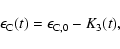
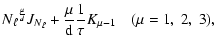
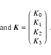
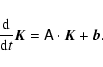
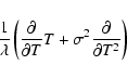
However, AGB stars have convective turbulent stellar envelopes, in which the stellar pulsations are generated and fluctuating thermodynamic conditions must be expected. Since no quantitative information about the strength of the related temperature fluctuations is at hand, we treat the root mean square (rms) temperature deviation
and the correlation time
as free parameters and investigate their influence on dust formation.
Our approach is based on a phenomenological, statistical description of the stochastic temperature fluctuations. The approach is based on the procedures developed by Gail et al. (1974), Gail & Sedlmayr (1974), and Gail et al. (1980). To be able to clarify and generalize the mathematic modelling, we use the theory of stochastic processes and stochastic differential equations in our investigation. We derive a system of Fokker-Planck equations for the one-point distribution function, which indicates the joint probability of a certain state of dust formation and temperature at a given time.
This Fokker-Planck system was solved in a gas box for a typical trajectory of a volume element in a stellar wind, to determine how strong the temperature fluctuations had to be to influence the dust condensation in an AGB wind significantly, and on what timescales the stochastic condensation process can be modelled in the microturbulent limit case. A microturbulent description was found to be admissible for correlations times lower than 104 s and rms-temperature deviations even as small as 20 K had a remarkable influence on the condensation process. Since the longest time steps in the dynamical code used in this work are of the order of several 103 s, this means that all fluctuations occuring on a sub-grid scale can be modelled by the microturbulent limit case. Therefore, in this work, a one-parametric microturbulent description of the stochastical dust condensation is developed and implemented into the CHILD-Code, a dynamical 1D-code that self-consistently solves the equations of hydrodynamics, thermodynamics, and time-dependent dust condensation, including a grey radiative transfer and an equilibrium chemistry for the species that are most important to dust condensation. The implementation of the presented sub-grid model into other numerical models for AGB winds, such as multidimensional models (e.g. Woitke 2006) or models including a frequency-dependent radiative transfer (e.g. Gautschy-Loidl et al. 2004), should be straightforward.
This paper develops a methodological approach to a theory of dust formation and growth under stochastic temperature fluctuations, introduced by Dirks (2000), with preliminary studies by Dirks (1993), Dirks & Sedlmayr (1998), and the studies of Schirrmacher & Dirks (2003), Schirrmacher et al. (2004) and Schirrmacher et al. (2005), and continues with the quantitative investigations of dust formation by Schirrmacher (2007).
In Sect. 2, we describe the deterministic dust formation theory, upon which this work is based. In Sect. 3, we describe our stochastical model for the temperature fluctuations and derive a system of Fokker-Planck equations, which describes dust formation under the influence of temperature fluctuations. In Sect. 4, we present a set of gas box calculations, where the influence of the fluctuation parameters in an AGB-like environment is investigated. The derivation of a fast microturbulent approach and its implementation into a self-consistent dynamical code for AGB winds, and our results and discussion are presented in Sect. 5. Our summary, conclusions, and perspective on future work are provided in Sect. 6.
We describe the dust component by a grainsize distribution function. This choice restricts our study to homogeneous dust grains, which consist of a number of identical monomers. However, growth processes including several growth species can be considered, provided that they result in the addition of an i-mer to the grain. Since the focus of this work is on the general impact of fluctuations on the condensation process and not on the detailed chemical composition of the grains, this approach seems adequate. We consider carbon grains with C, C2, C2 H, and C2 H2 as growth species.
We apply the moment method developed by Gail et al. (1984),
Gail & Sedlmayr (1988), and Gauger et al. (1990), which provides a set of equations for the moments  of the grain size distribution function
f(N,t) containing the number density
of the grain size distribution function
f(N,t) containing the number density![[*]](/icons/foot_motif.gif) of
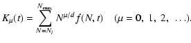
dust grains of size N (= number of monomers contained) at any given t. The moments
of f(N,t) are defined by:
of
dust grains of size N (= number of monomers contained) at any given t. The moments
of f(N,t) are defined by:
 |
(1) |
, and d is the spatial
dimension of the grains, which by assuming spherical particles we set to be d=3 in this work. The first four moments have an immediate physical interpretation:
 of grains of size
 :
:
 |
(2b) |
 |
(2c) |
 |
(2d) |
 of monomers condensed into grains of size
:
of monomers condensed into grains of size
:
 |
(2e) |

 is the undepleted carbon abundance of the dust free gas. Formation, growth, and evaporation of the dust are described by a two-step process: first, seed particles need to be formed, and subsequently, these particles grow by capturing more monomers from the gas phase. The formation of seed particles is assumed to be given by the stationary nucleation rate J*, calculated according to classical nucleation theory (see Gail et al. 1984, and references therein), whereas the net growth of the particles is assumed to occur by homogeneous growth, chemical growth, thermal evaporation, and chemical sputtering as calculated by Gail & Sedlmayr (1988) and Gauger et al. (1990).
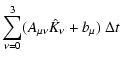
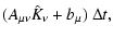
The time evolution in the first four dust moments is then given by
(see Gauger et al. 1990)
 is the creation/destruction rate of clusters of size
 .
It is assumed that
corresponds to the stationary nucleation rate J*, and
.
It is assumed that
corresponds to the stationary nucleation rate J*, and  corresponds to the net growth rate, i.e. including the effects of dust destruction.
Mathematically, Eq. (4a) is a closing condition for the equation
system Eq. (4b), so that the moments with negative  do not
have to be evaluated.
do not
have to be evaluated.
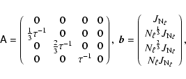
We introduce
The moment method presented in the previous section can be applied to all
astrophysical systems in which dust formation and growth occur in a
previously dust-free environment. The nucleation rate J and net growth
rate
are functions of the gas temperature
 ,
the dust temperature
,
the dust temperature
 ,
and the particle densities ni of the growth species.
,
and the particle densities ni of the growth species.
When adapting this method to various astrophysical environments, the time-dependent temperature und density structure must be provided, including the chemical particle densities of the growth species at any moment in time. Obviously, the particle densities of the growth species depend on the degree of condensation (see Eq. (3)). The temperature structure of the object usually also depends on the spatio-temporal dust distribution, because dust tends to dominate the energy exchange between a gas/dust mixture and any given radiation field. In dust-driven winds, the radiation pressure on the dust will be a dominant input term in the calculation of the hydrodynamical structure, i.e. the density profile.
The equation system Eq. (5) will conveniently become
part of the Fokker-Planck system Eq. (34) derived in
Sect. 3. It will therefore remain necessary to provide the
density, temperature, and particle densities of all growth species. Since a
coupled solution of the probabilistic set of equations and
hydrodynamic equations with radiative transfer would considerably increase the computation time,
we first performed some gas box studies, in which
we neglected the coupling to the hydrodynamic structure and radiative
transfer, and calculated the probabilistic dust formation on a prototype,
non-varying wind model described in Sect. 4. The results
of these gas box studies lead us to a microturbulent approach, which is suitable
for the implementation into the self-consistent dynamical wind calculations
presented in Sect. 5.
Since we have neither a concrete turbulence theory of stellar atmospheres, nor an observation-based quantitative knowledge concerning the irregular fluctuations, they must be analyzed using a statistical description, which accounts satisfactorily for fluctuations phenomenologically but does not include explicitly their physical causes.
The following approach therefore represents a formulation of the physics of dust formation in terms of stochastic processes, and a mathematical generalisation of physical problem constitutions as developed in the domain of line formation in random velocity fields, in particular by Gail et al. (1974), Gail & Sedlmayr (1974), and Gail et al. (1980). Within the concrete implementation, the fluctuation effect is limited to the temperature parameter without any restriction of the generality of this method, inasmuch as temperature is the most influential physical parameter with regard to dust formation and growth.
Further details of this approach and its mathematical background are given by Dirks (2000).
Within a stellar wind of velocity  ,
we describe generally
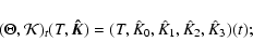
field quantities X in a gas volume element traveling radially towards the periphery of the circumstellar envelope, which at time t0 = 0 is situated at the surface of the star r= R*, by indicating the state X = X(t) within the comoving system. The temperature evolution can be described by a fluctuation conditional temperature deviation by the splitting of
,
we describe generally
field quantities X in a gas volume element traveling radially towards the periphery of the circumstellar envelope, which at time t0 = 0 is situated at the surface of the star r= R*, by indicating the state X = X(t) within the comoving system. The temperature evolution can be described by a fluctuation conditional temperature deviation by the splitting of
 into
into
 ,
where
,
where
 denotes the deterministic mean value of the
temperature and T(t) the stochastic temperature deviation.
denotes the deterministic mean value of the
temperature and T(t) the stochastic temperature deviation.
As is customary in probability theory, we consider, in the framework of a
statistical model, the determination (measurement) of the temperature deviation at time t in the gas element to be the random variable  .
Because of the significant dependence of both dust formation and growth on temperature, their
probabilistic state is described by a random variable
.
Because of the significant dependence of both dust formation and growth on temperature, their
probabilistic state is described by a random variable
 for the determination of the values of the dust
moments
for the determination of the values of the dust
moments
 .
The evolution in both temperature and dust, in the state space
.
The evolution in both temperature and dust, in the state space
 at each time,
will therefore be described by the family of random variables, given by the
time parameter t, i.e. by the stochastic process
at each time,
will therefore be described by the family of random variables, given by the
time parameter t, i.e. by the stochastic process
 ,
the paths of
which represent the possible evolutions
,
the paths of
which represent the possible evolutions
 designates the Borel sets of
 .
.
In view of the physical causes of the temperature fluctuations, it is
justified to assume the independence of the temperature fluctuations and
the present dust growth from the former temperature fluctuations as well as
the concrete genesis of the given dust particles. In that sense, the stochastic process
is ``without memory'', that is, for a given present state, both the past and
future of its physical development are statistically independent of each
other. With regard to the component of dust formation and growth in itself,
this process is indeed described by common differential equations of
first order (Eqs. (4a,b)), i.e. by a functional
connection in which the change in the system at time t depends only on
the state at this time, and not on former states. Altogether, we postulate that the stochastic process
 is a Markov process.
In terms of the fundamental theorem of Kolmogorov (see e.g. Arnold 1974, Theorem 1.8.1), a stochastic process is canonically given by a specified consistent family of finite-dimensional distributions, apart from stochastic equivalence. As for Markov processes, the finite-dimensional distributions are determined by indicating a start distribution and a transition probability, and the construction of the searched process is simplified by assuming the Markov-presupposition (see Arnold 1974, Chap. 2).
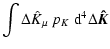
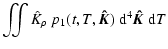
In the present case, we must determine the one-point probability
distribution to calculate the expectation values for dust formation
during temperature fluctuations; under the physically justified assumption of the continuous existence of probability densities, we therefore search for the density
 ,
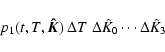
which, in the form
,
which, in the form
 |
(8) |
 and
and
 ,
indicates the probability that the fluctuation temperature reaches a value in the range
,
indicates the probability that the fluctuation temperature reaches a value in the range
![\( [T, T+\Delta T] \)](/articles/aa/full/2008/45/aa9243-07/img77.gif) and the dust formation moments reach a value in the range
and the dust formation moments reach a value in the range
![\( \left[ \hat{K}_{\mu} , \hat{K}_{\mu} + \Delta \hat{K}_{\mu} \right] \)](/articles/aa/full/2008/45/aa9243-07/img78.gif) .
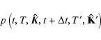
The stochastic information about this Markovian process from the transition probability density
.
The stochastic information about this Markovian process from the transition probability density
 |
(9) |
 at time
 ,
if it was found
in the state
,
if it was found
in the state
 at the previous time t. The
Chapman-Kolmogorov equation (also known as Einstein-Smoluchowski equation)
and all
at the previous time t. The
Chapman-Kolmogorov equation (also known as Einstein-Smoluchowski equation)
and all
 is considered to be the crucial characterizing feature of the transition
probabilities of Markov processes. By multiplication of
is considered to be the crucial characterizing feature of the transition
probabilities of Markov processes. By multiplication of
 and integration with respect to T1 and
 ,
Eq. (10) becomes the following
relation between the densities of the one-point distribution and the
Markovian transition probability density:
,
Eq. (10) becomes the following
relation between the densities of the one-point distribution and the
Markovian transition probability density:
 |
(11) |
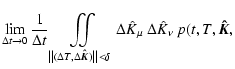
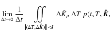
 in one term. We note
that the assumptions made about the existence and continuity of the partial
derivatives are fulfilled in our physical system.
and
in one term. We note
that the assumptions made about the existence and continuity of the partial
derivatives are fulfilled in our physical system.
and
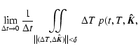
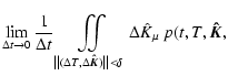
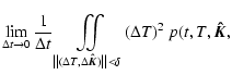
 are defined by the following infinitesimal moments, the existence of
which is as well presupposed as their independence of the special choice of
are defined by the following infinitesimal moments, the existence of
which is as well presupposed as their independence of the special choice of  within the derivation of Eq. (12):
 as a separation condition, that the transition probability density can be expressed in the form:
 .
pK describes the stochastics of dust formation
and its dependence on the fluctuation temperature at the initial time t. However, with respect to Eq. (5) and the
Markov-presupposition, it is independent of the temperature of the state at
time
.
.
pK describes the stochastics of dust formation
and its dependence on the fluctuation temperature at the initial time t. However, with respect to Eq. (5) and the
Markov-presupposition, it is independent of the temperature of the state at
time
.
The process component
 of the fluctuating temperature
deviation can be understood as the result of two factors: (i) if the
temperature in a gas volume element varies rapidly due to density
fluctuations caused by the collision interaction of particles, a relaxation
process will be initiated that results in a state of equilibrium with the
environment, assuming that the velocity of the change of
of the fluctuating temperature
deviation can be understood as the result of two factors: (i) if the
temperature in a gas volume element varies rapidly due to density
fluctuations caused by the collision interaction of particles, a relaxation
process will be initiated that results in a state of equilibrium with the
environment, assuming that the velocity of the change of
 in a linear approximation of the temperature behaviour depends only on T with
 ;
(ii) as an additional component including the turbulent temperature fluctuation, we have to assume a stochastically acting fluctuation force, which is supposed to be independent of
;
(ii) as an additional component including the turbulent temperature fluctuation, we have to assume a stochastically acting fluctuation force, which is supposed to be independent of  insofar as the probabilistic wave field is not considered physically dependent on the actual temperature deviation at the place of dust formation. Both terms together lead to an equation of the Langevin type:
 within the deterministic term
determines the order of magnitude of the relaxation time,
within the deterministic term
determines the order of magnitude of the relaxation time,
 ,
and the physical description of the temperature fluctuation has to be included in the definition of the stochastic term
,
and the physical description of the temperature fluctuation has to be included in the definition of the stochastic term
 .
The
chosen approach offers a wide range of possibilities for describing
temperature turbulences in different concrete physical situations. In the
prototype designed here, we assume the following characteristics of the
temperature fluctuation on the phenomenological level:
.
The
chosen approach offers a wide range of possibilities for describing
temperature turbulences in different concrete physical situations. In the
prototype designed here, we assume the following characteristics of the
temperature fluctuation on the phenomenological level:
Firstly, there is no reason to assume that  has a systematic effect on the temperature evolution; the behavior of the mean value
 is determined by the deterministic term, so that the expectation value equals:
 |
(16) |
 and
and
 for time spans
|t2 -t1| longer than the duration
for time spans
|t2 -t1| longer than the duration
 ,
which is characteristic of an individual
stochastic temperature modification, with
,
which is characteristic of an individual
stochastic temperature modification, with
 .
The
fluctuation force
.
The
fluctuation force
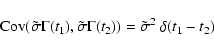
 produces a thermal noise at the place of dust formation by the influence of rapid fluctuations, i.e.
a purely random process for which the following expression, using the delta distribution, is valid:
produces a thermal noise at the place of dust formation by the influence of rapid fluctuations, i.e.
a purely random process for which the following expression, using the delta distribution, is valid:
 |
(17) |

 formally as stochastic process, we stipulate that the
one-point distributions (and consequently all finite-dimensional distributions) follow a Gaussian distribution with expectation value zero.
formally as stochastic process, we stipulate that the
one-point distributions (and consequently all finite-dimensional distributions) follow a Gaussian distribution with expectation value zero.
These requirements can only be fulfilled by a generalized random
process, i.e. in general by a continuous linear functional
 in the space
 of infinitely differentiable
functions
of infinitely differentiable
functions
 with bounded supports in
,
where
with bounded supports in
,
where
 is a random variable for each
  (see e.g. Gel'fand & Vilenkin 1964, Chap. III). More precisely, in the stochastic term of Eq. (15),
 has to be defined to be a generalized Gaussian process in which for every choice of linear independent functions
 the random variable
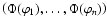 is normally distributed;
as can be verified, the phenomenal specifications are fulfilled
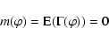
by white noise, i.e. for the average and covariance
functional of
we have:
is normally distributed;
as can be verified, the phenomenal specifications are fulfilled
by white noise, i.e. for the average and covariance
functional of
we have:
 |
(18a) |
 = =  |
|
= |
(18b) |
 .
The white noise, well-defined as a Gaussian process by the average and covariance functional, can be described as a distribution derivative of the generalization
.
The white noise, well-defined as a Gaussian process by the average and covariance functional, can be described as a distribution derivative of the generalization
 of the Wiener process Wt, which, being a homogeneous, stationary Gaussian Markov process, is well-known to be a model of the Brownian motion of a free particle (with Wt=0 for t<0):
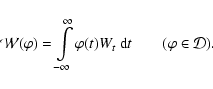 |
(19) |
 ,
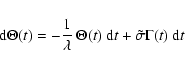
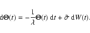
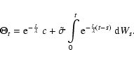
we can now define the special Langevin equation for the fluctuation
conditions within our prototype to be:
,
we can now define the special Langevin equation for the fluctuation
conditions within our prototype to be:
 |
(21) |
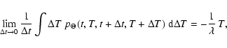
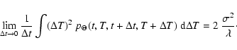
 a normally distributed random variable with expectation value 0, and by scaling its variance
by
a normally distributed random variable with expectation value 0, and by scaling its variance
by  ,
we calculate:
,
we calculate:
 ,
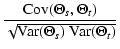
the root mean square temperature
fluctuation, indicates the mean turbulent temperature. Because of the
correlation function
,
the root mean square temperature
fluctuation, indicates the mean turbulent temperature. Because of the
correlation function
 has to be interpreted as the correlation time characteristic for the turbulence, i.e. the values of the parameter of the fluctuation
temperature in the gas element are only correlated within periods of time
approximately equal to the time taken to relax to temperature
equilibrium. The transition probability density of the Ornstein-Uhlenbeck
process can be directly calculated (cf. Todorovic 1992,
Propos. 3.7.3).
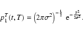
As we know from the theory of diffusion processes, for stochastic differential equations of the type Eq. (20) the searched moments in Eqs. (13a) and (13c) are produced directly from a proposition that holds for the terms of the stochastic differential equation (as drift vector and diffusion matrix, see Arnold 1974, Theorem 9.3.1):
has to be interpreted as the correlation time characteristic for the turbulence, i.e. the values of the parameter of the fluctuation
temperature in the gas element are only correlated within periods of time
approximately equal to the time taken to relax to temperature
equilibrium. The transition probability density of the Ornstein-Uhlenbeck
process can be directly calculated (cf. Todorovic 1992,
Propos. 3.7.3).
As we know from the theory of diffusion processes, for stochastic differential equations of the type Eq. (20) the searched moments in Eqs. (13a) and (13c) are produced directly from a proposition that holds for the terms of the stochastic differential equation (as drift vector and diffusion matrix, see Arnold 1974, Theorem 9.3.1):
For the determination of the transition probability density pK in Eq. (14), the following points must be considered.
Firstly, the stochastic nature of dust formation is due entirly to its dependence on the temperature fluctuation. Secondly, the
solution
 of
Eq. (6) for the initial value
of
Eq. (6) for the initial value
 transports the state
  at time t1 to the state
  at time t within the time period
t - t1.
at time t within the time period
t - t1.
With a canonical choice of random variables (which is always possible as a
corollary of the fundamental theorem of Kolmogorov),
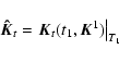
 for all t, the value of the random variables can, for small time steps
 ,
be set equal to the value
,
be set equal to the value
 |
(26) |
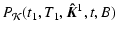
The probability
 of the transition from the state of process
 at time t1 to a state within the value set B at time t for sufficiently small time periods is therefore
 |
= |  |
|
| = | 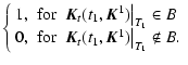 |
(27) |
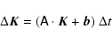 |
(28) |
 and using the -distribution, we obtain for the transition probability density:
In a conceptual respect, the analytical dependence of the dust formation moments according to Eq. (6) has now been transferred into a stochastic dependence of the random variables
 described by the transition probability density Eq. (29).
To specify the coefficient functions (Eq. (13)) within the Fokker-Planck equation Eq. (12), we calculate (and formulate by use of the summation convention):
.
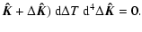
The Markovian property of pT and pK is carried forward to the entire process; the assumptions made in the derivation of the Fokker-Planck equation Eq. (12) are fulfilled, in particular the regularity assumptions for the partial derivative in Eq. (12), the existence of the moments Eq. (13) (even uncut), and the improbability of arbitrarily large fluctuations in the smallest time intervals: for any ,
we calculate:
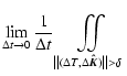 |
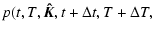 |
||
 |
(32) |
 determined in this way, we calculate for Eqs. (24), (25), (30), and (31), for the coefficient functions in Eq. (13) of the Fokker-Planck equation:
| BT | = | 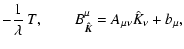 |
(33a) |
| AT | = | 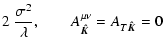 |
(33b) |
.
For the one-point probability density
the Fokker-Planck equation is then:
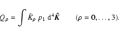
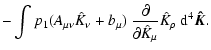
 we therefore define the first moment to be:
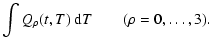
 to equation Eq. (34), we obtain:
 |
(36) |
 |
|||
 |
(37) |
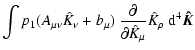
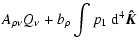
). For the second summand and its random variables,
we receive:
 |
= |  |
|
| = |  |
(38) |
-state space, which is in this case given by the Gaussian density of the Ornstein-Uhlenbeck process (with respect to the system Eq. (22)):
for
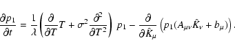
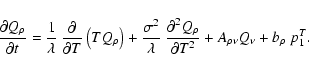
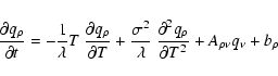
 is then given by the following coupled system of four second order linear partial differential equations of the parabolic type:
 ,
which constrain the dust formation in a probabilistic way:
.
,
which constrain the dust formation in a probabilistic way:
.
Since the local radiative acceleration is a function of the degree of
condensation  (
( ),
the direct application of the equation
system Eq. (43) to a wind description yields the problem
that different values of T would produce different accelerations for
different temperature deviations. The important feedback of the dust formation onto the underlying wind structure can therefore not be described using Eq. (43). If, however, the correlation length
of the fluctuations is so
small, that the process occurs at the microturbulent limit, this problem
can be evaded because the values of
),
the direct application of the equation
system Eq. (43) to a wind description yields the problem
that different values of T would produce different accelerations for
different temperature deviations. The important feedback of the dust formation onto the underlying wind structure can therefore not be described using Eq. (43). If, however, the correlation length
of the fluctuations is so
small, that the process occurs at the microturbulent limit, this problem
can be evaded because the values of  are then almost equal for all values of T. To determine i) for which values of ,
the stochastic dust formation can be described in the microturbulent limit case; and ii) for which values of ,
a significant influence of fluctuations on the dust formation can be expected, we applied the formalism described in Sect. 3 to a set of gas-box models, which present typical trajectories of volume elements in a stationary AGB wind. For the reasons stated above, no feedback of the dust formation on the hydrodynamical structure of the model is included. We assumed a constant wind velocity of 20 km s-1, which corresponds to a typical end velocity of an AGB wind. This assumption is required because the solution of the Fokker-Plank system Eq. (43), based on a more realistic wind model of velocity v(r) that increases with distance r, produces almost complete condensation in the slow part of the wind; this is due to the lack of consideration of the effect of radiative acceleration on the newly formed grains, which then causes them to become unrealistically long in the region of efficient dust condensation.
We adopted a high carbon-to-oxygen ratio, which, in turn, facilitates the dust formation process in the artificial situation.
In these prototypic calculations, we aim to constrain the parameter space of
and ,
and estimate the influence of the temperature fluctuations on the dust formation under AGB conditions; this would enable us to implement consistently the effects of the temperature fluctuations on dynamical model calculations as presented in Sect. 5.
are then almost equal for all values of T. To determine i) for which values of ,
the stochastic dust formation can be described in the microturbulent limit case; and ii) for which values of ,
a significant influence of fluctuations on the dust formation can be expected, we applied the formalism described in Sect. 3 to a set of gas-box models, which present typical trajectories of volume elements in a stationary AGB wind. For the reasons stated above, no feedback of the dust formation on the hydrodynamical structure of the model is included. We assumed a constant wind velocity of 20 km s-1, which corresponds to a typical end velocity of an AGB wind. This assumption is required because the solution of the Fokker-Plank system Eq. (43), based on a more realistic wind model of velocity v(r) that increases with distance r, produces almost complete condensation in the slow part of the wind; this is due to the lack of consideration of the effect of radiative acceleration on the newly formed grains, which then causes them to become unrealistically long in the region of efficient dust condensation.
We adopted a high carbon-to-oxygen ratio, which, in turn, facilitates the dust formation process in the artificial situation.
In these prototypic calculations, we aim to constrain the parameter space of
and ,
and estimate the influence of the temperature fluctuations on the dust formation under AGB conditions; this would enable us to implement consistently the effects of the temperature fluctuations on dynamical model calculations as presented in Sect. 5.
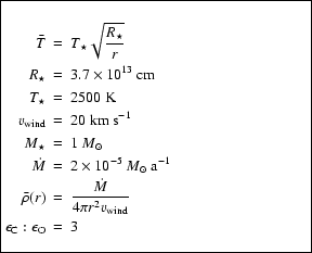
The gas-box wind model (see box) is used as input to the Fokker-Planck
system Eq. (43). We assume that at a
given moment in time t1, the densities
 are coupled
adiabatically along the T-axis.
are coupled
adiabatically along the T-axis.
These gas box models can be interpreted most effectively as the temporal development of the dust component in a volume
comoving with the given wind:
We start the integration at  and t=0 in a dust-free
situation. The Fokker-Planck system Eq. (43) is then
integrated forward in time with the Cranck-Nicolson method. Using
and t=0 in a dust-free
situation. The Fokker-Planck system Eq. (43) is then
integrated forward in time with the Cranck-Nicolson method. Using
 ,
the functions
and
,
the functions
and
 are used as input for the transition probabilities. By discretization with a second-order difference scheme, the Fokker-Planck system finds its numerical analogon in a
set of linear systems of equations, which can be represented by a tridiagonal matrix and then solved by a standard solver. Along the axis of the temperature fluctuation (T-axis), we truncated the integration domain at
are used as input for the transition probabilities. By discretization with a second-order difference scheme, the Fokker-Planck system finds its numerical analogon in a
set of linear systems of equations, which can be represented by a tridiagonal matrix and then solved by a standard solver. Along the axis of the temperature fluctuation (T-axis), we truncated the integration domain at
 ,
with
,
with
 ;
an integration from
;
an integration from  to
to  is numerically impossible and physically meaningless. The integration domain must be selected to be sufficiently large to ensure that the boundary conditions have no influence on those parts of the domain that contribute significantly to the Gaussian-weighted averaged expectation values. As a boundary condition, we used the corresponding deterministic path, and note that other non-pathological choices produced the same results.
In most calculations
(Sects. 4.1-4.3), we assumed
the dust temperature  to equal the gas temperature
 .
This corresponds to assuming an effective
energy exchange between gas and dust, e.g. slow fluctuations (large
), high densities (i.e. high collision rates). To
estimate the effects of dust temperature deviating from gas
temperature, we performed a set of calculations assuming
.
This corresponds to assuming an effective
energy exchange between gas and dust, e.g. slow fluctuations (large
), high densities (i.e. high collision rates). To
estimate the effects of dust temperature deviating from gas
temperature, we performed a set of calculations assuming
 ,
which could be interpreted as rapid fluctuations in a thin gas (see
Sect. 4.4).
,
which could be interpreted as rapid fluctuations in a thin gas (see
Sect. 4.4).
We solved the equation system Eq. (43) on top of the gas-box wind model described above. In Sects. 4.1 and 4.2, we present two parameter studies for  and .
In Sect. 4.3, we discuss the behaviour of the solution compared with a set of purely deterministic calculations for the same wind model. In Sect. 4.4, we present some models, where we assumed the dust temperature to remain at the mean temperature with the gas temperature continuing to fluctuate.
and .
In Sect. 4.3, we discuss the behaviour of the solution compared with a set of purely deterministic calculations for the same wind model. In Sect. 4.4, we present some models, where we assumed the dust temperature to remain at the mean temperature with the gas temperature continuing to fluctuate.
![\begin{figure}
\par\includegraphics[width=8.5cm,clip]{9243fg01.eps}\end{figure}](/articles/aa/full/2008/45/aa9243-07/img219.gif) |
Figure 1:
Parameter study for various mean turbulent temperatures .
Top panel: mean temperature (dotted) and mean density (logarithmic, solid). Panel 2: average nucleation rate (black, full: 20 K, dotted: 40 K, dashed 60 K, grey: deterministic model). Panel 3: average net growth rate. (The deterministic curve is covered by the black curve for
 K.) Panel 4: expectation value of the number density of dust grains (logarithmic). Panel 5: expectation value of the degree of condensation. K.) Panel 4: expectation value of the number density of dust grains (logarithmic). Panel 5: expectation value of the degree of condensation.
 s for all plots. s for all plots. |
| Open with DEXTER | |
The results of a study of different values of ,
i.e.
root mean square turbulent temperatures, are shown in
Fig. 1. In the top panel, the mean values of the radial
temperature and density structure are given; these values are used as input of
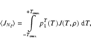
the calculation (see box in the head of this section). In Panels 2 and 3, the
mean nucleation rate
 and the mean net
growth rate
and the mean net
growth rate
 are plotted, which correspond to an
integration of
are plotted, which correspond to an
integration of
 and
and
 over
all T-paths weighted by the probability function
p1T(T) (see
Eq. (39)):
over
all T-paths weighted by the probability function
p1T(T) (see
Eq. (39)):
 |
(44a) |
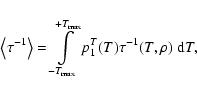 |
(44b) |
and
are evaluated at the gas temperature
 |
(45a) |
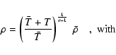 |
(45b) |
 |
(45c) |
 and
and
 are
calculated from the solutions
of the Fokker-Planck system
Eq. (43). The functions J and
are calculated at every time step using the given thermodynamical structure as input and the q3-solution of the Fokker-Planck system, which couples back into the equations by means of the depleted carbon concentration
are
calculated from the solutions
of the Fokker-Planck system
Eq. (43). The functions J and
are calculated at every time step using the given thermodynamical structure as input and the q3-solution of the Fokker-Planck system, which couples back into the equations by means of the depleted carbon concentration
 .
.
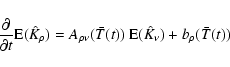
For small rms-temperature fluctuations, the models approach the behaviour of the deterministic calculation, as can be seen in Panels 2-5. This is the expected behaviour because using for example the sequence
 |
(48) |
 -distribution, it can be seen that the probability distribution of the Ornstein-Uhlenbeck process (cf. Eq. (39)) converges towards the -distribution for small widths :
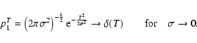 |
(49) |
 |
(50) |
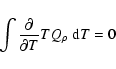 |
(51) |
 |
(52) |
 .
.
The most important physical effect of the fluctuations is the earlier onset of nucleation (panel 2), which becomes more pronounced with increasing .
The earlier onset of the nucleation is a direct consequence of the
lower temperature in the cool paths, which facilitates nucleation. In the
cool paths seeds are therefore produced, when
 ,
resulting in non-zero values for the ,
which persist after fluctuations, because these grains do not re-evaporate until S drops below 1 (see also Fig. 3).
The early nucleation is also obvious in Panel 4: high number densities of dust grains are reached about 0.5 R* deeper inside the wind, for
,
resulting in non-zero values for the ,
which persist after fluctuations, because these grains do not re-evaporate until S drops below 1 (see also Fig. 3).
The early nucleation is also obvious in Panel 4: high number densities of dust grains are reached about 0.5 R* deeper inside the wind, for
 K than for
K. The final particle size, however, will decrease with the enhanced nucleation rate J, because the condensable material is condensed into more individual grains and further condensation is stopped by depletion of the gas phase.
K than for
K. The final particle size, however, will decrease with the enhanced nucleation rate J, because the condensable material is condensed into more individual grains and further condensation is stopped by depletion of the gas phase.
![\begin{figure}
\par\includegraphics[width=8.5cm,clip]{9243fg02.eps}\end{figure}](/articles/aa/full/2008/45/aa9243-07/img242.gif) |
Figure 2:
Parameter study for various correlation times. The depicted quantities are identical to Fig. 1. Grey: deterministic; black full:
s; dotted: 107 s; dashed: 108 s; long dashed: 109 s.
K for all plots. |
| Open with DEXTER | |
![\begin{figure}
\par\includegraphics[width=11cm, angle=270,clip]{9243fg03.ps}\end{figure}](/articles/aa/full/2008/45/aa9243-07/img245.gif) |
Figure 3:
Degree of condensation
( top) and number density of dust grains ( bottom) along the T-r-plane in the deterministic ( right) and the stochastic ( left) case. T is the temperature deviation from the mean temperature (see Fig. 1 top panel). K0 and q0 are again normated to the total number density of hydrogen cores
 .
q0 ( bottom left) results from the first moment Eq. (35) of .
q0 ( bottom left) results from the first moment Eq. (35) of  via Eq. (42). The
K0 on the right are the result of a set of independent deterministic calculations along the single paths
via Eq. (42). The
K0 on the right are the result of a set of independent deterministic calculations along the single paths
 ,
i.e. there is no coupling along the T-axis in the deterministic case ( right). The degree of condensation ,
i.e. there is no coupling along the T-axis in the deterministic case ( right). The degree of condensation
 or
or
 must be understood accordingly,
 K, K,
 s). s). |
| Open with DEXTER | |
Panel 5 shows that the region of runaway condensation via growth of the existing grains is shifted about 0.25 R* inward for
K with respect to
K.
The slightly lower growth rate for
K with respect to that of the
K-model, can be explained by the earlier depletion, due to the larger amount of condensed material.
The results of a study of various values of the correlation time
of fluctuations with a rms-temperature fluctuation
 K are shown in Fig. 2.
In general, the dependence of the model calculations on the correlation time is rather small. We observe a slower decline in the nucleation rate for long correlation times (panel 2), alltough the overall impact of this effect on the dust moments (panels 4 and 5) is small.
We can identify two extreme cases, (i) the microturbulent limit (
 ); and (ii) the macroturbulent limit case (
 ). Mathematically, it is the operator
.
Since
 represents the part of dust formation for which the temperature deviation is in the interval
 ,
the Fokker-Planck operator describes the interaction between these different modes of the turbulence (cf. e.g. Traving 1975, Sect. 4).
,
the Fokker-Planck operator describes the interaction between these different modes of the turbulence (cf. e.g. Traving 1975, Sect. 4).
In a microturbulent situation, the influence of the operator, and with it, the influence of the fluctuation, become overwhelming. Physically, this implies that the fluctuations are rapid compared with the processes controlling the dust physics and are therefore uncorrelated on the (longer) timescales governing the condensation process. The different temperature paths are then strongly coupled (cf. Eq. (23)). In this case, it should be possible to find an easier way of calculating the influence of the temperature fluctuations, than the method presented here, because the -dependence vanishes. It can indeed be seen in Fig. 2 that the expectation values of the degree of condensation
(panel 5) are nearly identical for
s and
 s.
s.
The
-plots for
s and
 s in
Fig. 2 are also almost identical. They represent the macroturbulent limit case for which the
correlation time of the fluctuation is very long compared with the timescales
governing the condensation process, i.e. the interaction between the
different temperature paths is weak. Due to the slow relaxation, the gas volume element remains at the offset temperature in
the case of temperature disturbance. The separation of modes causes a quasi-deterministic behaviour of the expectation values. In the mathematical macroturbulent limit, the operator (53) vanishes and the Fokker-Planck system Eq. (43) for
corresponds to the deterministic system Eq. (6) for
s in
Fig. 2 are also almost identical. They represent the macroturbulent limit case for which the
correlation time of the fluctuation is very long compared with the timescales
governing the condensation process, i.e. the interaction between the
different temperature paths is weak. Due to the slow relaxation, the gas volume element remains at the offset temperature in
the case of temperature disturbance. The separation of modes causes a quasi-deterministic behaviour of the expectation values. In the mathematical macroturbulent limit, the operator (53) vanishes and the Fokker-Planck system Eq. (43) for
corresponds to the deterministic system Eq. (6) for  .
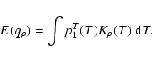
The expectation values of
then become the weighted mean of the deterministic moments ,
integrated over all temperature paths:
.
The expectation values of
then become the weighted mean of the deterministic moments ,
integrated over all temperature paths:
 |
(54) |
-values.
Figure 3 shows a comparison between the stochastic calculation (solution of the Fokker-Planck system Eq. (43), left hand side) and a set of deterministic calculations (solution of Eq. (6), right hand side) on the same
 /
/ -structure. In contrast to the solutions
of the Fokker-Planck system, we note that the deterministic plot on the right side represents a set of isolated calculations of the
for each path of constant temperature deviation T, i.e. the
do not ``interact'' along the T-axis.
-structure. In contrast to the solutions
of the Fokker-Planck system, we note that the deterministic plot on the right side represents a set of isolated calculations of the
for each path of constant temperature deviation T, i.e. the
do not ``interact'' along the T-axis.
![\begin{figure}
\par\includegraphics[width=12cm, angle=270,clip]{9243fg04.ps}\end{figure}](/articles/aa/full/2008/45/aa9243-07/img258.gif) |
Figure 4:
Net growth rate ( top) and nucleation rate ( bottom) for deterministic ( right) and stochastical calculations respectively. The stochastic plots on the left are coupled by the chemical consumption of monomers, i.e. by the q3-solution of the Fokker-Planck system Eq. (43) on the T-r-plane, whereas on the right - we again plot a sample of deterministic calculations.
K,
s.) |
| Open with DEXTER | |
Due to the choice of boundary conditions, the boundary paths (
)
of the stochastic system are identical to the corresponding
deterministic paths. However, Figs. 3 and 4
show clearly that the influence of the boundaries on the solutions
along the (t,T)-plane is weak; we note in particular the rapidly diminishing influence of the high temperature boundary visible in the lower left panel of Fig. 4. The influence of the boundaries on the expectation values is even orders of magnitudes smaller, because the
are weighted by the Gaussian-bell-shaped probability function pT, (see Eqs. (46), (47), and (39)).
Figure 4 shows the net growth rate (top) and nucleation rate
(bottom) in the stochastic (left) and deterministic cases (right). Both
plots look very similar, because the only coupling mechanism along the
T-axis (in the stochastic case) is the modified carbon abundance, which results from the modified degrees of condensation via the stochastic transport of  by the first two terms on the right side of
Eq. (43).
The similarity of the growth rate (upper plots in
Fig. 4) is the consequence of the fact that the depicted growth
rate is the hypothetical rate at which a grain would grow, if it were
present. This rate usually peaks before efficient nucleation begins (see
Fig. 1), and the peak in the growth rate in
Fig. 4 is therefore hardly influenced by the stochastical fluctuations,
even though it dominates the plot. For the same reason, the stochastic
nucleation rates (bottom left in Fig. 4) are not modified in
the part before (or inside) of their peak. Only after efficient nucleation
occurs at least somewhere in the integration domain, can the coupling
mechanism in terms of
be established; for values of
by the first two terms on the right side of
Eq. (43).
The similarity of the growth rate (upper plots in
Fig. 4) is the consequence of the fact that the depicted growth
rate is the hypothetical rate at which a grain would grow, if it were
present. This rate usually peaks before efficient nucleation begins (see
Fig. 1), and the peak in the growth rate in
Fig. 4 is therefore hardly influenced by the stochastical fluctuations,
even though it dominates the plot. For the same reason, the stochastic
nucleation rates (bottom left in Fig. 4) are not modified in
the part before (or inside) of their peak. Only after efficient nucleation
occurs at least somewhere in the integration domain, can the coupling
mechanism in terms of
be established; for values of
 (i.e. behind the peak in the nucleation rate, for
T < 0), the difference between the stochastic and deterministic cases
(bottom right) can indeed be seen.
(i.e. behind the peak in the nucleation rate, for
T < 0), the difference between the stochastic and deterministic cases
(bottom right) can indeed be seen.
We now consider more carefully the influence of the temperature
fluctuations. The location at which the net growth rate becomes positive is always closer to the star than the location at which nucleation from the gas phase initiates. This is easily understood because (hypothetical) dust grains should grow for
 ,
whereas the nucleation of new grains from the gas phase requires a supersaturation
,
whereas the nucleation of new grains from the gas phase requires a supersaturation
 .
.
If fluctuations are present, i.e. if the different T-paths are coupled by the Fokker-Planck system Eq. (43), the grains that nucleate in the cooler paths are mixed into the hotter paths, where they will grow as long as S > 1. The fluctuations therefore generate a mechanism that retains nuclei in a thermodynamic domain, where, in a deterministic situation, nucleation would not occur, due to a lack of supersaturation. This effect is clearly visible in Fig. 3: both, the number density of dust particles q0 and the degree of condensation
begin to rise earlier and reach their final level earlier in each path of the stochastic calculation (left) than in the corresponding path of the deterministic calculation (right).
The nucleation and growth rates depend sensitively on differences between gas and dust temperature, because in statistical equilibrium the creation rate increases with the gas temperature, while the corresponding evaporation rate increases with the temperature of the grain (see Patzer et al. 1998). Figure 5 shows model calculations where we assume that the dust temperature
remains at the mean temperature  of the deterministic model (panel 1), while the gas temperature fluctuates stochastically, as in the previous models.
The effects are significant. We note that the assumed rms temperature fluctation
was varied only between 1 K and 20 K. This calculation represents the upper limit of the possible influence of temperature fluctuations on dust formation; this is because the assumed thermal decoupling between the gas and dust maximises the temperature difference between the gas and dust, having a tremendous effect on the dust growth rates (see e.g. Patzer et al. 1998).
The assumption that a non-fluctuating dust temperature equals the deterministic mean temperature may correspond to assuming that a dust grain is affected by an undisturbed stellar radiation field. This picture appears plausible for large grains in a thin gas. In terms of our model approach, this implies, that the assumption of
 might be justified for the net growth rate. The size of the critical cluster, however, will generally not be large in the regions where remarkable nucleation takes place: we therefore expect this assumption to overestimate the influence of the fluctuation on the nucleation rate.
A realistic calculation of the temperature of the critical cluster would require the solution of the detailed balance between the (frequency-dependent) radiative heating and cooling rates, and the corresponding heating and cooling rates by means of inelastic collisions with the gas.
![\begin{figure}
\par\includegraphics[width=8.5cm,clip]{9243fg05.eps}\end{figure}](/articles/aa/full/2008/45/aa9243-07/img265.gif) |
Figure 5:
Parameter study for various mean turbulent temperatures ,
.
The presented quantities are the same as in Fig. 1. For panels 2-5: grey line: deterministic model (close to the full black line), full black line:  K, dotted: K, dotted:
 K, dashed: K, dashed:
 K, long dashed
K; K, long dashed
K;
 s for all plots. s for all plots. |
| Open with DEXTER | |
To calculate the dynamical wind models, we used the CHILD-Code developed by Fleischer et al. (1992). The CHILD-Code is a 1D-hydro code, which solves the coupled equation system of hydrodynamics, thermodynamics, equilibrium chemistry, time-dependent dust nucleation, growth, and evaporation, and grey radiative-transfer with spherical symmetry. Studies using the CHILD-Code were presented by e.g. Fleischer et al. (1992), Winters et al. (1994), Fleischer et al. (1995), Winters et al. (1995), Arndt et al. (1997), Winters et al. (1997), Schirrmacher et al. (2003), and Jeong et al. (2003).
In this work, two model families were calculated. The first model family
was calculated using the
version of the code described by Winters et al. (1997), whereas for the second
model family the version of the code presented by Schirrmacher et al. (2003) was used.
The difference between these two approaches relates to the different descriptions of the thermodynamic state and cooling functions.
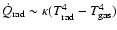
In the version from Winters et al. (1997) (henceforth referred to as model
family 1) assumes a monoatomic ideal gas of constant molecular weight and
analytical cooling function
 .
In contrast, the second model family (henceforth model family 2) uses tabulated state and cooling functions
.
In contrast, the second model family (henceforth model family 2) uses tabulated state and cooling functions
 ,
which
were calculated by assuming statistical equilibrium (SE) in the relevant
excitational states of the relevant species (for details
see Woitke et al. 1996a,b; Schirrmacher et al. 2003).
,
which
were calculated by assuming statistical equilibrium (SE) in the relevant
excitational states of the relevant species (for details
see Woitke et al. 1996a,b; Schirrmacher et al. 2003).
These two model families were chosen because the results of Sect. 4.4 suggested that differences between the dust and gas temperatures might be of particular importance to assessing the impact of the temperature fluctuations. In the CHILD-Code, the dust temperature is set to be the radiation temperature; the possible differences between gas and dust temperature are therefore sensitive to the cooling behaviour of the gas. Model family 1 was calculated for rapid radiative relaxation towards radiative equilibrium, whereas model family 2 was calculated with a more sophisticated input physics, which allowed for considerable local deviations between gas and radiation temperature.
In the deterministic case, Eqs. (4) are implemented in a straightforward way into the dynamical model calculation for the cases of dust growth and evaporation. The problem of dust destruction, i.e. the shrinking of dust grains by evaporation to sizes below  ,
requires special treatment because the destruction rate is not primarily a function of the state variables of the gas, but
depends clearly on the dust distribution function f(N,t)itself. In the CHILD-Code, the dust destruction rate is therefore
obtained by means of detailed book-keeping of the dust growth history, as
described by Gauger et al. (1990). This procedure cannot be applied to the
stochastical treatment presented in Sect. 3, because it is impossible to reconstruct a reasonable grain size distribution function f(N,t) from the conditional probabilities
obtained by the solution of the Fokker-Planck system Eq. (43). This circumstance has to be taken into account when designing an implementation of stochastical dust formation in time-dependent model calculations.
,
requires special treatment because the destruction rate is not primarily a function of the state variables of the gas, but
depends clearly on the dust distribution function f(N,t)itself. In the CHILD-Code, the dust destruction rate is therefore
obtained by means of detailed book-keeping of the dust growth history, as
described by Gauger et al. (1990). This procedure cannot be applied to the
stochastical treatment presented in Sect. 3, because it is impossible to reconstruct a reasonable grain size distribution function f(N,t) from the conditional probabilities
obtained by the solution of the Fokker-Planck system Eq. (43). This circumstance has to be taken into account when designing an implementation of stochastical dust formation in time-dependent model calculations.
Fortunately, the results presented in Sect. 4 revealed two important features of the implementation of the method into a dynamical framework:
remained almost unaffected, - see Fig. 1 and note the logarithmic scale in the plot for J (panel 2), in contrast to the linear scale in the plot for
(panel 3);
of the fluctuation, is
admissible.
 ,
obtained by solving the Fokker-Planck
system Eq. (43) in a static environment for given gas temperature
,
obtained by solving the Fokker-Planck
system Eq. (43) in a static environment for given gas temperature
 ,
density
,
density  ,
carbon abundance
,
and rms-temperature deviation
which is the only remaining parameter describing the fluctuation. Figure 7 shows the resulting microturbulent nucleation rates for two different values of
and the deterministic reference (left plot).
,
carbon abundance
,
and rms-temperature deviation
which is the only remaining parameter describing the fluctuation. Figure 7 shows the resulting microturbulent nucleation rates for two different values of
and the deterministic reference (left plot).
Table 1:
Range and spacing of the 3D-tables containing the microturbulent nucleation rates
 .
.
.
Consequently, the tables were calculated with fewer grid points in the -direction (see Table 1). Figure 6 shows slices of the tabulated
for various values of at typical values for
and
during the onset of dust formation in an AGB wind. The
peak value of the nucleation rate decreases slightly with increasing fluctuation strength, whereas the onset of nucleation is shifted towards
considerably higher temperatures.
![\begin{figure}
\par\includegraphics[width=8cm,clip]{9243fg06.eps}\end{figure}](/articles/aa/full/2008/45/aa9243-07/img272.gif) |
Figure 6:
-study for
for
 g/cm-3 and g/cm-3 and
 .
K (solid line), 20 K (dotted), 40 K (dashed) and 60 K (long dashed). .
K (solid line), 20 K (dotted), 40 K (dashed) and 60 K (long dashed). |
| Open with DEXTER | |
![\begin{figure}
\par\mbox{\includegraphics[width=6cm,clip]{9243fg07.eps} \include...
...ip]{9243fg08.eps} \includegraphics[width=6cm,clip]{9243fg09.eps} }\end{figure}](/articles/aa/full/2008/45/aa9243-07/img276.gif) |
Figure 7:
The microturbulent nucleation rate  in a
/
in a
/
 plane for
 ,
i.e.
C/O ,
i.e.
C/O  1.8. The temperature is given in Kelvin and the density in g cm-3. The dashed lines correspond to nucleation rates of 1.8. The temperature is given in Kelvin and the density in g cm-3. The dashed lines correspond to nucleation rates of
 and -25. The dots correspond to the grid points in the calculation. Left: deterministic rate, middle:
K, right:
K.
and -25. The dots correspond to the grid points in the calculation. Left: deterministic rate, middle:
K, right:
K. |
| Open with DEXTER | |
There are two main advantages of this approach in implementing the effects of temperature fluctuations in dynamical model calculations:
vanishes. This has the advantages that, i) the dimension of the tables for
is reduced by one, which allows superior numerical resolution in the remaining dimensions; and ii) there is no need for a self-consistent description of the correlation times of the fluctuations;
 ,
if grains are formed during a temporary
temperature deviation, they will not be destroyed, when the undisturbed situation is restored. This situation can occur in the cooling flow of an AGB wind just before deterministic nucleation begins. This earlier (i.e. at higher mean temperatures) onset
of nucleation in the presence of temperature fluctuation is described properly by our microturbulent nucleation rate. An overestimation of this effect is avoided, since in the case that the mean
thermodynamic conditions leads to an evaporation of macroscopic grains
(S<1), the deterministic net growth rate
will prevent the
formation of dust grains.
,
if grains are formed during a temporary
temperature deviation, they will not be destroyed, when the undisturbed situation is restored. This situation can occur in the cooling flow of an AGB wind just before deterministic nucleation begins. This earlier (i.e. at higher mean temperatures) onset
of nucleation in the presence of temperature fluctuation is described properly by our microturbulent nucleation rate. An overestimation of this effect is avoided, since in the case that the mean
thermodynamic conditions leads to an evaporation of macroscopic grains
(S<1), the deterministic net growth rate
will prevent the
formation of dust grains.
Table 2:
Overview over the model parameters of the dynamical wind calculations.
 is a parameter for the temperature dependence of the dust opacity (see Gail & Sedlmayr 1987).
Table 3:
Relative changes
 )
of the mass-loss rates under
the influence of the temperature fluctuations.
)
of the mass-loss rates under
the influence of the temperature fluctuations.
A set of over 200 dynamical wind models was calculated. The model parameters are summarized in Table 2. The results of all model calculations are listed in Tables 4 and 5.
For model family 1, the models with
 K (models 6, 13, and 16), as well as particularly compact stars (
 K, and
 ), had numerical problems at the beginning when the first shock front steepened in the hydrostatic start model. The corresponding models are omitted in Table 4.
Model family 2 is calculated using a more sophisticated
gas model (see Schirrmacher et al. 2003) based on a statistical
equilibrium (SE) calculation of all relevant particle
densities and excitation levels of atoms, electrons, molecules, and ions in a radiation field parametrised by the radiation temperature
 ,
and a local hydrodynamic environment parametrised by an average velocity gradient
,
and a local hydrodynamic environment parametrised by an average velocity gradient
 .
These models can show remarkable differences between
and
.
These models can show remarkable differences between
and
 ,
due to the slower cooling behaviour and inclusion of the dissociation energy of H2 into the caloric equation of state (for details see Schirrmacher et al. 2003).
,
due to the slower cooling behaviour and inclusion of the dissociation energy of H2 into the caloric equation of state (for details see Schirrmacher et al. 2003).
Table 4: Mass-loss rates and final velocities for models with T4-cooling, ideal gas, (model family 1).
Table 5: Mass-loss rates and final velocities, models with tabulated NLTE-cooling and state functions, (model family 2).
For models with strong fluctuations (
K), the calculation was often aborted during the first shock increase in the hydrostatic start model, for both model families. This can usually be avoided by some fine-tuning of the numerical parameters that control the time steps.
However, to ensure that we had a coherent sample for the quantitative evaluation, no individual fine-tuning was completed and the corresponding models are omitted or marked with (-) in Tables 4
and 5.
![\begin{figure}
\par\mbox{\includegraphics[width=8.8cm,clip]{9243fg10.eps} \includegraphics[width=8.8cm,clip]{9243fg11.eps} }
\end{figure}](/articles/aa/full/2008/45/aa9243-07/img504.gif) |
Figure 8:
Snapshots from the dynamical model calculations at t = 90 P, model 12, NLTE-cooling,
 K-1. Left: deterministic, right:
K. Represented quantities: top panel: velocity v (solid), particle density of hydrogen cores
(dotted), the small ticks indicate the positions of the grid points. Panel 2: gas temperature
(dotted), radiation temperature
(solid). Panel 3: nucleation rate J (dotted), net growth rate
(solid). Panel 4: degree of condensation
(solid), radiative acceleration K-1. Left: deterministic, right:
K. Represented quantities: top panel: velocity v (solid), particle density of hydrogen cores
(dotted), the small ticks indicate the positions of the grid points. Panel 2: gas temperature
(dotted), radiation temperature
(solid). Panel 3: nucleation rate J (dotted), net growth rate
(solid). Panel 4: degree of condensation
(solid), radiative acceleration  (dotted).
 |
| Open with DEXTER | |
In Fig. 8, a comparison of a typical snapshot of the resulting wind structures for the deterministic and stochastic model is presented. The earlier onset of nucleation in the case including fluctuations (right figure) can be seen in panel 4. However, in these two - as in most other models - the impact of the temperature fluctuations is of a quantitative, rather than qualitative nature. Therefore, a statistical evaluation of the resulting mass loss rates was performed.
The mass loss rate was chosen for the quantitative evaluation, because i) it is the most important wind quantity in the evolution of the star, and the material injection into the surrounding ISM; and ii) it is obtained by averaging the wind structure over a comparably long period of time, so that the impact of numerical noise can be averaged.
The mass loss rates in Tables 4
and 5 were obtained by averaging the mass loss rate at
 from periods 90-120. The averaging process was started at
P=90 to ensure that all disturbances from the starting phase,
where the forced piston-oscillation of the velocity at the inner boundary
was increased to its final amplitude, and the hydrostatic
starting model had to evolve to the quasi-stationary situation, have
had sufficient time to travel to the outer boundary of the model.
from periods 90-120. The averaging process was started at
P=90 to ensure that all disturbances from the starting phase,
where the forced piston-oscillation of the velocity at the inner boundary
was increased to its final amplitude, and the hydrostatic
starting model had to evolve to the quasi-stationary situation, have
had sufficient time to travel to the outer boundary of the model.
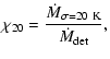
In the quantitative evaluation, the ratios between the stochastic and
deterministic mass loss rates were calculated according to
 |
(55) |
 K. These quantities are presented in the rightmost column of Tables 4 and 5.
The
 were averaged separately for the two model families and the two different dust extinction coefficients
.
The
results are shown in Table 3.
were averaged separately for the two model families and the two different dust extinction coefficients
.
The
results are shown in Table 3.
For model family 1 (ideal gas, analytical T4-cooling), a clear trend for
the mass-loss rates increasing with the fluctuation strength can be
seen. This tendency is valid for both values of the dust extinction, but appears to be stronger for the higher values of
,
which is the
expected result. The onset of nucleation at lower temperatures facilitates
dust formation, resulting in a higher mass loss. The increase in this
effect with a stronger coupling of the dust to the accelerating radiation
field also appears reasonable. The statistical basis for the values of  is however poor. However, when studying models 10,
11, or 14, for which the calculation achieved completion for
K, and
is however poor. However, when studying models 10,
11, or 14, for which the calculation achieved completion for
K, and
 could not be calculated because the deterministic model
failed, the trend for mass loss rates increasing with
holds when
comparing the corresponding models with
,
or 40 K.
could not be calculated because the deterministic model
failed, the trend for mass loss rates increasing with
holds when
comparing the corresponding models with
,
or 40 K.
For model family 2 (tabulated SE-state and cooling functions), the results
are not as clear. The scattering in the mass-loss rates of the particular
models was significantly higher, whereas the differences in the average values of
were smaller. In many cases, the inclusion of the fluctuations
even resulted in a decrease in the mass-loss rate, as for 3 of the 6 values
of
in Table 3.
We assume that the reason for the far less regular behaviour of this model
family is that the coupling in the equation system of the
dynamical formulation has a stronger non-linear character than for model
family 1. Effects such as the dissociation of hydrogen, and the dependence of the SE-radiative cooling rates on the chemical state of the gas are included in model family 2 (see Schirrmacher et al. 2003), and induce a strong non-linear behaviour, so that a clear trend in the influence of the temperature fluctuations on these models cannot be extracted from our calculations.
We have presented a time-dependent stochastic formulation of astrophysical dust formation under the influence of temperature fluctuations and a method to apply this to dynamical model calculations of dust-driven winds of AGB stars.
The formulation of the dust formation process by means of the theory of stochastic processes
has first produced a set of coupled Fokker-Plack equations replacing the deterministic
dust moment equations.
Since this formulation was technically not yet suited to the direct implementation in a dynamical wind calculation, we have investigated a set of gas-box models to determine i) the maximum timescale of correlation
time
that would prohibit a microturbulent formulation of the
stochastic dust formation; and ii) the order of the rms-temperature
deviation ,
for which a remarkable influence of the fluctuations on
the dust formation can be expected.
For values of
 s, the microturbulent
approximation was found to be valid, and for values of
s, the microturbulent
approximation was found to be valid, and for values of
 K, the influence of the temperature fluctuations on the dust formation was remarkable. The main influence of the temperature fluctuations on the dust formation was the fluctuation-induced nucleation in a region that remained dust-free in the deterministic case. Effective dust formation therefore occurred for a supersaturation ratio
 ,
i.e. the critical supersaturation ratio was lowered.
,
i.e. the critical supersaturation ratio was lowered.
Guided by the results of these gas-box calculations we proposed a microturbulent approach, easily implemented on a sub-grid level into dynamical model-calculations. A set of numerical model calculations using this microturbulent sub-grid model for the temperature fluctuations was also presented. The results showed a clear trend of massloss rates increasing with increasing fluctuation strength, close to LTE. Model calculations using a more sophisticated gas description with tabulated SE-state and cooling functions were too unreliable to establish such a trend.
The application of the presented microturbulent nucleation rate to other numerical codes for AGB winds is straightforward, as long as the deterministic code uses the moments of the dust distribution function for the description of the time evolution of the dust component.
The presented method for the stochastical description of dust formation under the influence of temperature fluctuations can be applied to other astrophysical situations, if a deterministic time-dependent formulation of the dust physics, based on moments of the grain-size distribution function, is available, which can be used for the determination of the transition probabilities and possibly as start and boundary values of the resulting Fokker-Planck system. To apply a microturbulent nucleation rate to other dust-forming astrophysical systems, it is necessary to investigate first the importance and timescales of correlation effects. This investigation could be completed using the methods presented in Sect. 4.
For completeness we make two further remarks:
Acknowledgements
The members of the Centre of Astronomy and Astrophysics (TU Berlin) are thanked for many fruitful discussions on the subject. In particular Dr. J. M. Winters is thanked for useful advises at the beginning of the project and Dr. B. Patzer, Dr. M. Hegmann, and Prof. Dr. W. Kegel for valuable comments. This work was partly supported by the DFG-SFB 555.