A&A 490, 501-514 (2008)
DOI: 10.1051/0004-6361:200810385
High accretion rates in magnetised Keplerian discs mediated by a Parker
instability driven dynamo
A. Johansen1,2 - Y. Levin1
1 - Leiden Observatory, Leiden University, PO Box 9513, 2300 RA Leiden, The Netherlands
2 -
Work partially done at Max-Planck-Institut für Astronomie, Königstuhl
17, 69117 Heidelberg, Germany
Received 13 June 2008 / Accepted 22 August 2008
Abstract
Hydromagnetic stresses in accretion discs have been the subject of intense
theoretical research over the past one and a half decades. Most of the disc simulations have assumed a small initial magnetic field and studied the turbulence that arises from the magnetorotational instability. However, gaseous discs in galactic nuclei and in some binary systems are likely to have
significant initial magnetisation. Motivated by this, we performed ideal magnetohydrodynamic simulations of strongly magnetised, vertically stratified discs in a Keplerian potential. Our initial equilibrium configuration, which has an azimuthal magnetic field in equipartion with thermal pressure, is unstable to the Parker instability. This leads to the expelling of magnetic
field arcs, anchored in the midplane of the disc, to around five scale heights
from the midplane. Transition to turbulence happens primarily through magnetorotational instability in the resulting vertical fields, although magnetorotational shear instability in the unperturbed azimuthal field plays a significant role as well, especially in the midplane where buoyancy is weak.
High magnetic and hydrodynamical stresses arise, yielding an effective  -value of around 0.1 in our highest resolution run. Azimuthal magnetic field expelled by magnetic buoyancy from the disc is continuously replenished by the stretching of a radial field created as gas parcels slide in the linear gravity field along inclined magnetic field lines. This dynamo process, where
the bending of field lines by the Parker instability leads to re-creation of
the azimuthal field, implies that highly magnetised discs are astrophysically
viable and that they have high accretion rates.
-value of around 0.1 in our highest resolution run. Azimuthal magnetic field expelled by magnetic buoyancy from the disc is continuously replenished by the stretching of a radial field created as gas parcels slide in the linear gravity field along inclined magnetic field lines. This dynamo process, where
the bending of field lines by the Parker instability leads to re-creation of
the azimuthal field, implies that highly magnetised discs are astrophysically
viable and that they have high accretion rates.
Key words: accretion, accretion disks - Galaxy: center - instabilities - magnetohydrodynamics (MHD) - turbulence
Since the seminal work of Balbus & Hawley (1991) it has been widely recognised that hydromagnetic stresses play a central role in the dynamics of Keplerian gaseous discs. Much of the subsequent theoretical work has been devoted to the study of the magnetic dynamo driven by a combination of magnetorotational instability (MRI), rotation, and Keplerian shear (Brandenburg et al. 1995; Hawley et al. 1996, see
Brandenburg & Subramanian 2005, for an excellent review of astrophysical
dynamo theory). Typically, numerical
simulations of the MRI-driven dynamo begin with an initial zero net flux magnetic field with an associated pressure which is a small fraction of the thermal pressure. The idea is that the MRI-driven turbulence should increase the characteristic coherence length of the magnetic field, and grow its mean strength to a significant fraction of the equipartition value. The simulations,
however, have had at best a mixed success in explaining high and persistent inflow rates observed in astrophysical accretion discs. Firstly, a number of recent numerical experiments have shown that the effectiveness of the dynamo depends in a critical way on the value magnetic Prandtl number, defined as the ratio of the collisional kinematic viscosity to the magnetic diffusivity
(Lesur & Longaretti 2007; Fromang et al. 2007, following suggestive non-disc simulations of Schekochihin et al. 2005 and a careful study of previously published MRI-turbulence results by Pessah et al. 2007).
The upshot of this work is that when the Prandtl number is significantly less
than one, as is expected in most accretion discs (Balbus & Henri 2008), the
dynamo seems to fail![[*]](/icons/foot_motif.gif) . Secondly, in the zero net flux simulations where
all parameters are chosen so that the dynamo works, the measured value of the
Shakura-Sunyaev parameter
is typically of order 10-3 and at most
10-2 (e.g. Fromang & Nelson 2006; Brandenburg et al. 1995; Johansen & Klahr 2005; Sano et al. 2004).
This is 1-2 orders of magnitude smaller than what is required to explain
the high accretion rates in dwarf novae systems (King et al. 2007).
. Secondly, in the zero net flux simulations where
all parameters are chosen so that the dynamo works, the measured value of the
Shakura-Sunyaev parameter
is typically of order 10-3 and at most
10-2 (e.g. Fromang & Nelson 2006; Brandenburg et al. 1995; Johansen & Klahr 2005; Sano et al. 2004).
This is 1-2 orders of magnitude smaller than what is required to explain
the high accretion rates in dwarf novae systems (King et al. 2007).
The weak initial magnetic fields assumed in almost all disc-MRI simulations may
be unrealistically small for many astrophysical discs. We give here two examples:
- 1.
- Extended accretion discs around central supermassive black holes (such
as the ones traced by megamasers in nearby galaxies; see e.g. Vlemmings et al. 2007; Greenhill 2007) are fed by molecular material in the interstellar medium. Molecular clouds are known to have large scale superthermal magnetic fields, and thus the initial magnetic fields in AGN discs
are likely to be comparable to or larger than the thermal equipartition values.
The
 2 pc molecular circumnuclear disc in our galactic centre is permeated
by large scale equipartition magnetic fields (Hildebrand et al. 1990; Wardle & Konigl 1990) which are certain to play an important dynamical role in its subsequent evolution.
2 pc molecular circumnuclear disc in our galactic centre is permeated
by large scale equipartition magnetic fields (Hildebrand et al. 1990; Wardle & Konigl 1990) which are certain to play an important dynamical role in its subsequent evolution.
- 2.
- Accretion discs in close binary systems, which are fed by a Roche-lobe overflow
from a tidally distorted low mass star, may be initially magnetised. The
magnetisation
 of the gas as it departs from the donor star can be
estimated as
of the gas as it departs from the donor star can be
estimated as
 |
(1) |
where  (measured in Gauss) is the stellar magnetic field at the
surface,
(measured in Gauss) is the stellar magnetic field at the
surface,  is the speed of sound at the stellar surface, and
  is the
density of gas as it becomes detached from the star. The density
can be estimated as
is the
density of gas as it becomes detached from the star. The density
can be estimated as
 |
(2) |
where  is the average accretion rate of the companion, and
  is the radius of the star. We get
 |
(3) |
The streaming and shearing motion after the gas detaches from the star can
further amplify the magnetic field. Clearly, there is a realistic parameter
range where the initial magnetisation is high.
Motivated by these astrophysical considerations, in this paper we perform
numerical experiments on gas discs which contain initially strong magnetic
fields, with magnetic pressure comparable to that of the gas. Specifically, we
initialise the azimuthal field so that it is subject to the Parker instability
(PI, Parker 1966) in the vertical stratification.
In terms of initial conditions our physical set up is close to Machida et al. (2000). However, Machida et al. (2000) focused on the formation and evolution of a disc corona, and the spirit or their numerical experiment was different from ours. They have simulated the whole circular
disc, and have introduced reflecting boundary conditions at the midplane of the disc, which suppresses field anchoring in the midplane. By contrast, our purpose is to understand the long-term dynamics of the disc, possible field confinement, and the dynamo processes related to strong magnetic fields. Therefore, our shearing-box simulations focus on a small part of the disc and
study it with high numerical resolution. We simulate the fluid both below and
above the midplane, and thus have no artificial boundary conditions at the midplane of the disc.
We find that both the short term and, more importantly, the long term behaviour of initially strongly magnetised discs is radically different from that of their weakly magnetised counterparts. We observe the following three-step dynamics: (a) the Parker instability expels azimuthal field in huge arcs, creating vertical field which becomes the seed for a strong magnetorotational
instability; (b) matter sliding down inclined field lines stretches the azimuthal
magnetic field and creates a vertically dependent large scale mean radial field; and (c) the Keplerian shear recreates azimuthal field from the stretching of the radial field. The latter step closes the dynamo cycle, in much the same way as was sketched by Tout & Pringle (1992) a decade and a half ago, although non-axisymmetric magnetorotational instability in the
azimuthal field also plays an important role in creating accretion stresses in
our simulations (Foglizzo & Tagger 1995; Balbus & Hawley 1992; Terquem & Papaloizou 1996). The
azimuthal field remains strongly concentrated towards the disc midplane; this is in contrast with the simulations of Parker instability which do not include strong Keplerian shear in the radial direction (Kim et al. 1998). We show that the dynamo is robust and stable over at least tens of orbital periods, and that the accretion torque increases if we use a finer grid. We observe
-values as high as 0.1 in our highest resolution run.
The plan of the paper is as follows. In Sect. 2 we detail the mechanics of our numerical experiments, and in the following section (Sect. 3) we test our computer code by comparing the results of Parker instability simulations without Keplerian shear to the extensive literature that exists on the PI under rigid rotation. In Sect. 4 we
perform simulations with the Keplerian shear included, and present our main
results. We devote the next section (Sect. 5) to analysing the
confinement of azimuthal flux to the disc by a dynamo process. In Sect. 6 we conclude with the discussion of the astrophysical implications and possible future improvements of our work.
2 Description of the numerical experiment
In this section we describe the numerical method we use to solve the equations
of ideal magnetohydrodynamics, the set up of an initial condition that is
unstable to the Parker instability, and technical issues such as dissipation
terms and boundary conditions. We use the Pencil
Code to
solve the relevant partial differential equations.
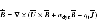
We consider a local corotating patch of a Keplerian accretion disc. The coordinate axes are oriented such that x points radially away from the central gravity source, y points along the main orbital flow, while z points vertically out of the disc parallel to the Keplerian rotation vector
 .
In the shearing sheet approximation the equation of motion, for the velocity field
.
In the shearing sheet approximation the equation of motion, for the velocity field  relative to the Keplerian flow, is
Here
 is the shear parameter, with q=0 for rigid rotation and q=3/2 for Keplerian rotation. The left hand side includes advection both by the velocity field
itself and by the linearised Keplerian flow
is the shear parameter, with q=0 for rigid rotation and q=3/2 for Keplerian rotation. The left hand side includes advection both by the velocity field
itself and by the linearised Keplerian flow
 .
The first two terms on the right hand side represent the Coriolis force in the x- and y-directions,
modified in the y-component by the radial advection of the Keplerian flow,
.
The first two terms on the right hand side represent the Coriolis force in the x- and y-directions,
modified in the y-component by the radial advection of the Keplerian flow,
 .
The third term is the linearised vertical component of the gravity of the central object, while the Lorentz and pressure gradient forces appear in the usual way. The high order
numerical scheme of the Pencil Code has very little numerical dissipation from
time-stepping the advection term (Brandenburg 2003), so we add explicit
viscosity through the term
.
The third term is the linearised vertical component of the gravity of the central object, while the Lorentz and pressure gradient forces appear in the usual way. The high order
numerical scheme of the Pencil Code has very little numerical dissipation from
time-stepping the advection term (Brandenburg 2003), so we add explicit
viscosity through the term
 ,
described in detail in Sect. 2.2.
,
described in detail in Sect. 2.2.
In this paper we consider stratified models with 4-16 orders of magnitude of range in densities. In low-density regions the Alfvén speed
 |
(5) |
may become very high when strong magnetic fields are transported away from regions near the midplane to form a low density corona, and we must reduce  artificially in order to avoid very low time-steps in the explicit numerical scheme of the Pencil Code. We have done so by replacing the density
in the Lorentz force
term of Eq. (4) by a modified density
artificially in order to avoid very low time-steps in the explicit numerical scheme of the Pencil Code. We have done so by replacing the density
in the Lorentz force
term of Eq. (4) by a modified density  defined as
![\begin{displaymath}%
\frac{1}{\rho^*} = \frac{1}{\rho}
\left[1+\left(\frac{v_{\rm A}^2}{M^2}\right)^n \right] ^{-1/n}\cdot
\end{displaymath}](/articles/aa/full/2008/41/aa10385-08/img39.gif) |
(6) |
Here M is a limiting value for the Alfvén speed and n is an index that
smooths the transition from the regime where the Alfvén speed is not affected
(
 )
to the region where the limiter applies (
)
to the region where the limiter applies (
 ). This
yields an effective Alfvén speed
). This
yields an effective Alfvén speed
 in the limit
 ,
while in the limit of high Alfvén speeds the effective speed is
,
while in the limit of high Alfvén speeds the effective speed is
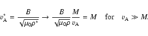 |
(7) |
We used a smoothing index of n=5. We are grateful to Heinemann for implementing this form of the Alfvén limiter in the Pencil Code (Heinemann et al. 2007). A similar Alfvén speed limiter was used by Miller & Stone (2000). The Alfvén limiter in the form presented here does not conserve momentum, but we have experimented with
 and
and
 and found no qualitative differences in our results. Thus we apply
to all 2D simulations, and
to the
3D simulations to get a longer time-step in those computationally expensive runs.
and found no qualitative differences in our results. Thus we apply
to all 2D simulations, and
to the
3D simulations to get a longer time-step in those computationally expensive runs.
The magnetic vector potential  is evolved through the induction equation
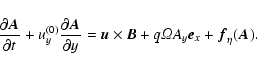 |
(8) |
The explicit resistivity term
 is discussed in Sect. 2.2. Working with the vector potential
rather than the magnetic field
is discussed in Sect. 2.2. Working with the vector potential
rather than the magnetic field  has the advantage that
 is kept solenoidal (
 )
by mathematical construction. The stretching of the radial component of the magnetic field by the Keplerian shear
is represented by the second term on the right hand side of Eq. (8) (Brandenburg et al. 1995). The current density
)
by mathematical construction. The stretching of the radial component of the magnetic field by the Keplerian shear
is represented by the second term on the right hand side of Eq. (8) (Brandenburg et al. 1995). The current density  ,
needed for the Lorentz force in Eq. (4), is calculated from Ampère's law
,
needed for the Lorentz force in Eq. (4), is calculated from Ampère's law
 .
We set the vacuum permeability
.
We set the vacuum permeability  .
.
The mass density is evolved in its logarithmic form
 |
(9) |
The last term on the right hand side is an explicit diffusion term (see Sect. 2.2). It is advantageous to evolve the logarithmic mass density when a large dynamical range in density is considered. Also, in the initial magnetohydrostatic equilibrium,  varies parabolically with z, and the Pencil Code's finite difference approach to spatial derivatives
yields a perfect derivative of parabolic curves (Brandenburg 2003).
varies parabolically with z, and the Pencil Code's finite difference approach to spatial derivatives
yields a perfect derivative of parabolic curves (Brandenburg 2003).
We close the dynamical equation system by applying an isothermal equation of state with
 .
The sound speed
is assumed constant.
.
The sound speed
is assumed constant.
2.2 Dissipation terms
The viscosity term
 of Eq. (4) appears in full generality as
![$\displaystyle %
{\vec f}_\nu = \nu_3
\left[\nabla^6{\vec u}+({\vec S}^{(3)}\cdo...
...bla}\ln\rho)\right]
+ {\vec \nabla}\nu_{\rm shock}({\vec \nabla}\cdot{\vec u}).$](/articles/aa/full/2008/41/aa10385-08/img60.gif) |
|
|
(10) |
The viscosity includes both hyperviscosity with coefficient  and shock viscosity with coefficient
 .
A simplified third order rate-of-strain tensor
.
A simplified third order rate-of-strain tensor
 is here defined as
 |
(11) |
The shock viscosity coefficient is obtained by taking the negative part of the
divergence of ,
then taking the maximum over three grid cells in each
direction, and finally smoothing over three grid cells, to obtain
![\begin{displaymath}%
\nu_{\rm shock}=c_{\rm shock} \langle {\rm max}[-{\vec \nabla}\cdot{\vec u}]_+ \rangle
(\delta x)^2.
\end{displaymath}](/articles/aa/full/2008/41/aa10385-08/img65.gif) |
(12) |
Here
 is a parameter of order unity (Haugen et al. 2004).
For the resistivity term
 in Eq. (8) we include both
hyperresistivity and shock resistivity,
in Eq. (8) we include both
hyperresistivity and shock resistivity,
 |
|
|
(13) |
This form is the resistivity conserves all components of the magnetic field .
We set
 .
.
Mass diffusion consists of shock diffusion,
![$\displaystyle %
{\vec f}_D(\ln\rho) = D_{\rm shock} [\nabla^2\ln\rho+({\vec \nabla}\ln\rho)^2] + {\vec \nabla}
D_{\rm shock}\cdot{\vec \nabla}\ln\rho,$](/articles/aa/full/2008/41/aa10385-08/img70.gif) |
|
|
(14) |
where
 is defined in Eq. (12). We also
upwind the finite differencing of the advection term in the continuity equation
(Dobler et al. 2006). Mass diffusion and upwinding are necessary to damp out
spurious small scale modes that are left behind due to the dispersion error in
the finite differencing of the advection term in the continuity equation.
is defined in Eq. (12). We also
upwind the finite differencing of the advection term in the continuity equation
(Dobler et al. 2006). Mass diffusion and upwinding are necessary to damp out
spurious small scale modes that are left behind due to the dispersion error in
the finite differencing of the advection term in the continuity equation.
We set shock diffusivity coefficients to
 in all simulations to dissipate energy in shocks forming far away
from the midplane of the disc. In run S3D_256_Lz18, which is extended
vertically compared to the other 3-D simulations, we had to double
to dissipate enough energy in the regions above six scale heights from
the midplane.
in all simulations to dissipate energy in shocks forming far away
from the midplane of the disc. In run S3D_256_Lz18, which is extended
vertically compared to the other 3-D simulations, we had to double
to dissipate enough energy in the regions above six scale heights from
the midplane.
We test the dependence of our results on dissipation parameters by keeping the
mesh Reynolds number approximately constant with increasing resolution, i.e. scaling hyperdissipation parameters by
 and shock dissipation
parameters by
and shock dissipation
parameters by
 .
Higher resolution simulations thus probe the
effect of decreasing the dissipation coefficients.
.
Higher resolution simulations thus probe the
effect of decreasing the dissipation coefficients.
Table 1:
Simulation parameters.
2.3 Initial conditions
We assume that the initial magnetic field is toroidal, a reasonable assumption
since Keplerian shear efficiently generates coherent toroidal field from a
small radial component. Furthermore, we tune the initial field so that (a)
magnetic pressure is the constant fraction
 of the gas pressure,
and (b) vertical hydrostatic equilibrium is enforced, i.e.
of the gas pressure,
and (b) vertical hydrostatic equilibrium is enforced, i.e.
 |
(15) |
Mathematically, the initial density, magnetic field, and vector potential are
given by
Here
 is the gas scale height,
and
is the gas scale height,
and  is the initial density in the midplane. The thermal pressure
alone would give rise to a scale height of
is the initial density in the midplane. The thermal pressure
alone would give rise to a scale height of
 .
We
will use this more familiar scale height as our unit of length, setting H=1throughout the paper.
.
We
will use this more familiar scale height as our unit of length, setting H=1throughout the paper.
Since we shall consider many (six to twelve) scale heights above and below the
midplane, we run into the problem that the finite differencing of the magnetic
pressure gradient underestimates its actual value and leads to spurious
accelerations far away from the midplane. This is not a problem for the
equilibrium density stratification, since the logarithmic density varies as a
parabola with height over the midplane, and any parabolic shape has a perfect
numerical derivative in the symmetric finite difference scheme of the Pencil
Code. In order to give magnetic stratification equal opportunity as the
density, and to obtain a perfect initial magnetohydrostatic equilibrium, we
measure magnetic field and current density relative to their initial values, as
explained below.
We split the field and the current into two components, as follows. For the
Lorentz force in Eq. (4) and the induction term in Eq. (8) we replace
| |
|
 |
(19) |
| |
|
 |
(20) |
The initial magnetic field
 is given by Eq. (17),
while the initial current density
is given by Eq. (17),
while the initial current density
 is calculated as
|
Jx(0)(z) |
= |
 |
|
| |
= |
![$\displaystyle \sqrt{2\mu_0^{-1}\beta^{-1} c_{\rm s}^2 \rho_0} [z/(2 H_\beta^2)]
\exp[-z^2/(4 H_\beta^2)].$](/articles/aa/full/2008/41/aa10385-08/img106.gif) |
(21) |
The effect of this splitting is that the initial, mean field is not exposed to
any (numerical or explicit) resistivity. Since we wish for resistive effects to
go to zero with increasing resolution, the splitting does not introduce any extra spurious effects. We have
checked that the Parker instability develops similarly in models with and
without this field splitting, and have found that the models without splitting
indeed converge towards the models with splitting as the resolution increases.
![\begin{figure}
\par\includegraphics[width=8.4cm,clip]{0385fi1a.eps}\hspace*{2mm}...
....eps}\hspace*{2mm}
\includegraphics[width=8.4cm,clip]{0385fi1d.eps}\end{figure}](/articles/aa/full/2008/41/aa10385-08/Timg107.gif) |
Figure 1:
Evolution of the Parker instability in 2D rigid rotation (run R2D_256). Overlaid on the density are magnetic field streamlines (white lines) and velocity field vectors (white arrows, averaged over 8 grid points, the longest arrows represent approximately four times the sound
speed). The initial stratification is unstable to magnetic buoyancy, and magnetic field arcs begin to rise from the midplane. The arcs merge to form longer arcs, and eventually the system settles down into a new equilibrium state with two superarcs and four dense pockets of matter in
the midplane. |
| Open with DEXTER |
We perturb the initial Keplerian velocity field by Gaussian noise of
amplitude
 .
This perturbation seeds the linear Parker
instability, and the noise also contains leading waves that can be amplified by
non-axisymmetric magnetorotational instability in the azimuthal magnetic field
in simulations with Keplerian shear.
.
This perturbation seeds the linear Parker
instability, and the noise also contains leading waves that can be amplified by
non-axisymmetric magnetorotational instability in the azimuthal magnetic field
in simulations with Keplerian shear.
We set the usual shearing sheet boundary conditions in the x and y directions (shear-periodic in x and periodic in y). At the upper and lower boundaries we impose free-slip conditions,
 ,
for the velocity field
and perfect conductor,
,
for the velocity field
and perfect conductor,
 ,
for the magnetic vector potential .
This effectively
allows the radial and azimuthal components of the magnetic field to evolve
freely at the upper and lower boundary planes, while the vertical component of
the magnetic field is forced to be zero. Globally the average value of all
components of the magnetic field are then conserved. Perfect conductor boundary
conditions do not allow azimuthal flux to flow out of the box, and therefore
there is a concern that the presence of the boundaries will artificially
enhance the field in the disc. To address this concern, we have made sure that
our results have converged with increasing vertical extent of the box; see
Sect. 5 and Figs. 7 and 12.
,
for the magnetic vector potential .
This effectively
allows the radial and azimuthal components of the magnetic field to evolve
freely at the upper and lower boundary planes, while the vertical component of
the magnetic field is forced to be zero. Globally the average value of all
components of the magnetic field are then conserved. Perfect conductor boundary
conditions do not allow azimuthal flux to flow out of the box, and therefore
there is a concern that the presence of the boundaries will artificially
enhance the field in the disc. To address this concern, we have made sure that
our results have converged with increasing vertical extent of the box; see
Sect. 5 and Figs. 7 and 12.
For the mass density
we set a symmetric boundary condition with
 at the upper and lower boundaries. Although this
precludes the gas pressure gradient from participating in magnetohydrostatic
equilibrium there, the free-slip boundary condition for the velocity field,
with zero vertical velocity component, means that this does not cause any
unwanted accelerations.
at the upper and lower boundaries. Although this
precludes the gas pressure gradient from participating in magnetohydrostatic
equilibrium there, the free-slip boundary condition for the velocity field,
with zero vertical velocity component, means that this does not cause any
unwanted accelerations.
We perform a series of simulations of the evolution of Parker and
magnetorotational instabilities, usually starting from an equipartition
( )
accretion disc in magnetohydrostatic equilibrium (as described in
Sect. 2.3). Simulation parameters are written in Table 1. The
main runs are the shearing sheet simulations S3D_*, representing varying
resolution (S3D_256, S3D_512), higher initial ratio of gas to magnetic
pressure (S3D_256_b3), increased vertical extent of the box (S3D_256_Lz18) and
an exploration of the effect of a moderate amount of net vertical field (S3D_256_Bz0.03). For testing purposes we also run a series of 2D and 3D rigid rotation simulations (R2D_256, R2D_512, R2D_256_Lz24, R3D_256), which we present in the next section.
)
accretion disc in magnetohydrostatic equilibrium (as described in
Sect. 2.3). Simulation parameters are written in Table 1. The
main runs are the shearing sheet simulations S3D_*, representing varying
resolution (S3D_256, S3D_512), higher initial ratio of gas to magnetic
pressure (S3D_256_b3), increased vertical extent of the box (S3D_256_Lz18) and
an exploration of the effect of a moderate amount of net vertical field (S3D_256_Bz0.03). For testing purposes we also run a series of 2D and 3D rigid rotation simulations (R2D_256, R2D_512, R2D_256_Lz24, R3D_256), which we present in the next section.
3 Testing the code: evolution of the Parker instability under rigid
rotation
In this section we study the evolution of the ``pure'' Parker instability in 2D and 3D simulations without shear (Parker 1966; Kim et al. 1997). This allows us to test our code against the previously published results, and to review previous work done on the evolution of the Parker instability in systems with no systematic shear.
Basu et al. (1997) performed 2D inertial frame simulations of the non-linear evolution of the Parker instability. They found that primarily antisymmetric midplane crossing modes are excited by the random noise initial condition. The instability develops quickest in the tenuous gas high over the midplane. As the magnetic field lines rise in big arcs, matter streams unobstructed down the
lines that are no longer horizontal. Dense pockets of gas (approximately a factor two times more dense than the average state) form in the midplane, anchoring the rising magnetic field lines there. The final state of the Parker instability, in which the tension in the bent magnetic field lines balances the buoyancy, has a lower energy than the initial equilibrium state
(Mouschovias 1974) and is therefore preferred.
In Fig. 1 we show the evolution of the Parker instability obtained with the Pencil Code under rigid rotation in the 2D (y,z) plane (run R2D_256). Magnetic field lines initially rise in arcs of wavelength
 .
As matter streams sideways along the rising
field lines (see arrows in Fig. 1) dense clumps of gas appear in the
midplane after 10 orbits. Eventually the magnetic arcs merge and form two
superarcs with four dense gas clumps in the midplane.
.
As matter streams sideways along the rising
field lines (see arrows in Fig. 1) dense clumps of gas appear in the
midplane after 10 orbits. Eventually the magnetic arcs merge and form two
superarcs with four dense gas clumps in the midplane.
In Fig. 2 we show the maximum gas density in the box as a function of time. The clumps in the midplane are overdense by around factor 1.6-2.2 compared to the initial state, and this contrast is relatively well converged already at 256  128 grid points (as is the non-linear evolution of the Parker instability in general). Our simulations are in good qualitative
agreement with the Basu et al. (1997) simulations.
128 grid points (as is the non-linear evolution of the Parker instability in general). Our simulations are in good qualitative
agreement with the Basu et al. (1997) simulations.
In Fig. 3 we show the mean azimuthal magnetic field as a function of height over the midplane in the saturated state of the 2D Parker instability under rigid rotation. The initial azimuthal field is redistributed by the Parker instability so that some of the midplane flux ends above four scale heights from the midplane. This scale is similar to the typical azimuthal
wavelength of the Parker instability, so the final scale of vertical variation of the field likely comes about as the magnetic tension in the rising field lines grows to match the buoyant rise of the field lines. The non-linear transition from the initially stratified state to a state with magnetic arcs anchored in the midplane leads to the formation of an approximately force-free
corona extending from 4 scale heights from the midplane. In the corona, the magnetic tension and pressure terms are large (compared to their difference) and oppositely directed, and current flows parallel to the magnetic field lines. Increasing the vertical extent of the box from 12 to 24 scale heights leads to a transport of some magnetic flux to regions with |z|>6 H,
at the cost of a 20-30% decrease in the magnetic flux in the region |z|<6 H. The overall shape of the azimuthal magnetic field distribution is nevertheless relatively unchanged.
![\begin{figure}
\par\includegraphics[width=8.2cm,clip]{0385fig2.eps} \end{figure}](/articles/aa/full/2008/41/aa10385-08/Timg114.gif) |
Figure 2:
The maximum gas density as a function of time for 2D simulations of
the Parker instability (under rigid rotation). Increasing resolution leads
to no significant change of the maximum density, showing that the Parker
instability operates in a robust way already at 256
128 grid
points. |
| Open with DEXTER |
![\begin{figure}
\par\includegraphics[width=8.2cm,clip]{0385fig3.eps} \end{figure}](/articles/aa/full/2008/41/aa10385-08/Timg115.gif) |
Figure 3:
Mean azimuthal magnetic field, averaged over the y-direction, as a
function of height z over the midplane in 2D simulations with rigid
rotation. The initial Gaussian magnetic pressure
profile is lifted by the Parker instability, reducing the azimuthal flux by
a factor of approximately 1.5 in the midplane. The flux is transported to
above four scale heights from the midplane, and an approximately force
free corona develops at these high altitudes. Increasing the vertical
extent of the computational domain from 12 to 24 scale heights causes the
flux to be transported slightly further away from the midplane, but the
overall shape of the magnetic field distribution stays approximately the
same. |
| Open with DEXTER |
![\begin{figure}
\par\includegraphics[width=8.2cm,clip]{0385fig4.eps} \end{figure}](/articles/aa/full/2008/41/aa10385-08/Timg116.gif) |
Figure 4:
Mean azimuthal magnetic field versus height over the midplane for
the Parker instability in 3D rigid rotation. The azimuthal field quickly
spreads evenly over the entire vertical extent of the box, in contrast to
the 2D case (shown in Fig. 3) which makes a non-linear transition
to a state that still has azimuthal flux differences. |
| Open with DEXTER |
Two-dimensional models of the Parker instability allow only the undular mode to develop, but not the related interchange mode (Matsumoto et al. 1993), and hence the field has no possibility to escape from the disc. In three-dimensional rigidly rotating disc simulations, the
field does escape. In Fig. 4 we show the evolution of the azimuthal field in a 3D model including rotation (but still no shear). Now the azimuthal field quickly redistributes itself evenly with height over the midplane, leading to a state where vertical gravity is balanced only by thermal pressure. Allowing the mixed undular/interchange instability to take
place leads to a genuinely turbulent state (Kim et al. 1998), which mixes the
azimuthal field vertically and eventually spreads it uniformly throughout the entire extent of the box. In the next section we will show, however, that Keplerian shear completely suppresses the vertical spreading of the azimuthal field, which remains concentrated towards the disc midplane due to a dynamo coupling between Bx and By.
![\begin{figure}
\par\mbox{\includegraphics[width=1.5cm]{0385fi5a.eps} \includegra...
...1.5cm]{0385fi5g.eps} \includegraphics[width=8.8cm]{0385fi5h.eps} }
\end{figure}](/articles/aa/full/2008/41/aa10385-08/Timg117.gif) |
Figure 5:
The vertical magnetic field at the sides of the simulation box for
run S3D_512. The initial fastest growing wavelength of the Parker
instability is around 5 scale heights in the azimuthal direction and 0.5 scale heights in the
radial direction. The magnetorotational instability
eventually sets in as the vertical field grows in amplitude, and the box
turns turbulent with a strongly fluctuating vertical field. |
| Open with DEXTER |
The Parker instability in a shearing, rotating frame (which is the relevant
frame for most astrophysical purposes) must necessarily be more complicated
than in the rigidly rotating frame. The intrinsically non-axisymmetric instability is
deformed by the radial shear, while the whole coordinate frame can tap energy
from the gravitational potential through Maxwell and Reynolds stresses.
Already Shu (1974) expanded the Parker instability to include the effect of
shear. The conclusion of the analytical stability analysis is that no amount
of shear can completely stabilise against the Parker instability, as the
instability can develop at such small radial scales that growth happens faster
than shear.
4 The Parker instability in Keplerian shear
Having gained insight into the evolution of the Parker instability in 2D and
3D models with rotation but no shear, we now turn to the combined effect of
Parker and magnetorotational instabilities in a shearing sheet model of a
Keplerian accretion disc.
4.1 Creation of vertical field
In Fig. 5 we show the evolution of the vertical component of
the magnetic field at the sides of the box for run S3D_512. The following
sequence of events is observed: first the (sheared) Parker instability grows
unaffected by the MRI, but as the vertical magnetic fields gets a significant
amplitude, the MRI sets in and leads to a turbulent state where both PI and MRI
determine the dynamics. The Parker instability initially sets in high up in
the atmosphere where the buoyancy is strongest, at the typical wavelength
 and
and
 .
We actually observe that the radial
wavelength of the Parker instability decreases with increasing resolution as
the reduced dissipation allows growth at higher wave numbers. Eventually the
whole disc goes into a non-linear turbulent state with strongly fluctuating
vertical fields and twisted magnetic field loops extending far above the
midplane of the disc. The typical radial coherence scale in this state is much
longer than in the initial linear growth phase (compare
.
We actually observe that the radial
wavelength of the Parker instability decreases with increasing resolution as
the reduced dissipation allows growth at higher wave numbers. Eventually the
whole disc goes into a non-linear turbulent state with strongly fluctuating
vertical fields and twisted magnetic field loops extending far above the
midplane of the disc. The typical radial coherence scale in this state is much
longer than in the initial linear growth phase (compare
 to
to
 in Fig. 5).
The initial azimuthal field is also unstable to a (transient) non-axisymmetric magnetorotational ``instability'' (Keppens et al. 2002; Foglizzo & Tagger 1995; Balbus & Hawley 1992; Terquem & Papaloizou 1996).
Magnetorotational instability in the azimuthal field has highest growth rate
for modes with asmall vertical wavelength. The absence of high kz modes in the first panel of Fig. 5 indicates that non-axisymmetric MRI is not the dominant driver of the linear dynamics of the system. However, in Fig. 6 we show the vertical velocity field at the y=-Ly/2 plane for run S3D_512 during the linear growth phase. The top panel exhibits the usual signs of Parker instability high up in the atmosphere, but changing the contrast by two orders of magnitude (bottom panel) reveals modes of very short radial and vertical wavelength in the midplane of the disc, representing trailing waves that have already been amplified by magnetorotational instability in the azimuthal field. Transient amplification of swinging waves may also be important in determining the non-linear evolution of the system at later times (e.g. Lesur & Ogilvie 2008; Rincon et al. 2007).
![\begin{figure}
\par\includegraphics[width=7cm,clip]{0385fig6.eps} \end{figure}](/articles/aa/full/2008/41/aa10385-08/Timg123.gif) |
Figure 6:
The vertical velocity component at the y=-Ly/2 plane during
the linear phase of run S3D_512 (at
 ). The top panel
shows the high radial wavenumber structures typical for the 3D Parker
instability. However, changing the contrast by two orders of magnitude ( bottom panel)
reveals structures of high vertical wavenumber in the midplane of
the disc, likely a result of magnetorotational instability in the azimuthal
field. ). The top panel
shows the high radial wavenumber structures typical for the 3D Parker
instability. However, changing the contrast by two orders of magnitude ( bottom panel)
reveals structures of high vertical wavenumber in the midplane of
the disc, likely a result of magnetorotational instability in the azimuthal
field. |
| Open with DEXTER |
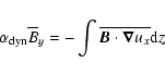
Although production of vertical field is not a main ingredient of azimuthal MRI, any unstable mode with a non-axisymmetric vertical velocity component can create significant vertical field by stretching the large scale azimuthal field (although highly variable in the vertical direction). The
production of large scale vertical field by the Parker instability, on the other hand, is demonstrated in Fig. 7. Here we plot the mean azimuthal field and the root-mean-square of the vertical field as a function of height over the midplane for the mixed PI/MRI shearing sheet simulations. Significant vertical magnetic fields of magnitude Bz
0.2 (with associated pressure  50) arise due to magnetic buoyancy.
There is a reversal of the azimuthal magnetic field at around four scale heights from the midplane. The correspondence between run S3D_256 and run S3D_256_Lz18 is extremely close, so the sign reversal is not due to the presence of the vertical boundary. Increasing resolution leads to some
increase in vertical field strength in the midplane, but the field reversal still takes place at the same height over the midplane. Although the non-linear state of the combined PI and MRI is time-dependent and fluctuating, there is a clear saturation and vertical confinement of the mean azimuthal magnetic field (we return to the issue of field confinement in
Sect. 5).
50) arise due to magnetic buoyancy.
There is a reversal of the azimuthal magnetic field at around four scale heights from the midplane. The correspondence between run S3D_256 and run S3D_256_Lz18 is extremely close, so the sign reversal is not due to the presence of the vertical boundary. Increasing resolution leads to some
increase in vertical field strength in the midplane, but the field reversal still takes place at the same height over the midplane. Although the non-linear state of the combined PI and MRI is time-dependent and fluctuating, there is a clear saturation and vertical confinement of the mean azimuthal magnetic field (we return to the issue of field confinement in
Sect. 5).
![\begin{figure}
\par\includegraphics[width=8.2cm,clip]{0385fig7.eps} \end{figure}](/articles/aa/full/2008/41/aa10385-08/Timg125.gif) |
Figure 7:
Confinement of the azimuthal field in shearing box simulations.
The mean azimuthal field and the root-mean-square of the vertical magnetic
field are plotted as a function of height over the midplane. The Parker
instability creates strong vertical fields from the initial azimuthal flux
(dotted line in top plot). Vertical loss of azimuthal flux is nevertheless
completely suppressed outside of a field reversal occurring at
approximately four scale heights from the midplane. Doubling the resolution (S3D_512) leads
to an increased vertical field strength and a decreased azimuthal field in
the midplane, likely due to a significant increase in turbulent motions at higher
resolution (see Table 2). |
| Open with DEXTER |
The magnetorotational instability in turn feeds off both the vertical
field lines created by the Parker instability and the azimuthal field component
still present in the non-linear state. The resulting Maxwell stress
 ,
averaged over time and radial and azimuthal directions, is
shown as a function of height over the midplane in Fig. 8. We
have divided the stress into contributions from the mean field,
,
averaged over time and radial and azimuthal directions, is
shown as a function of height over the midplane in Fig. 8. We
have divided the stress into contributions from the mean field,
 ,
and fluctuating
field,
,
and fluctuating
field,
 .
The occurrence of a large scale Bx is discussed in detail in
Sect. 5. The radial field couples with the large scale azimuthal
field to yield a large scale structure in the Maxwell stress as well,
relatively well converged when increasing the resolution.
.
The occurrence of a large scale Bx is discussed in detail in
Sect. 5. The radial field couples with the large scale azimuthal
field to yield a large scale structure in the Maxwell stress as well,
relatively well converged when increasing the resolution.
The fluctuating magnetic field is associated with significant stresses around
the midplane, with a Maxwell stress in the range
 in the
regions within a couple of scale heights from the midplane. The stress from
this fluctuating field increases significantly with increasing resolution, as
the decreasing dissipation on small radial scales allows the Parker instability
to create stronger vertical fields, while the decreased numerical and
artificial dissipation lets the both vertical field and azimuthal field MRI
develop faster.
in the
regions within a couple of scale heights from the midplane. The stress from
this fluctuating field increases significantly with increasing resolution, as
the decreasing dissipation on small radial scales allows the Parker instability
to create stronger vertical fields, while the decreased numerical and
artificial dissipation lets the both vertical field and azimuthal field MRI
develop faster.
![\begin{figure}
\par\includegraphics[width=8.1cm,clip]{0385fig8.eps} \end{figure}](/articles/aa/full/2008/41/aa10385-08/Timg133.gif) |
Figure 8:
The Maxwell stress
as a function of height
over the midplane. The top panel shows the stress from the mean field
 ,
while the bottom panel shows the
contribution from the fluctuating field ,
while the bottom panel shows the
contribution from the fluctuating field
 .
The magnetorotational
instability feeds off both the azimuthal fields and the large scale vertical
fields created by the Parker instability, to create significant stresses,
up to .
The magnetorotational
instability feeds off both the azimuthal fields and the large scale vertical
fields created by the Parker instability, to create significant stresses,
up to
 in the midplane of the high
resolution run S3D_512.
in the midplane of the high
resolution run S3D_512. |
| Open with DEXTER |
In Fig. 9 we show the measured mean Maxwell stress
as a function of time. The run S256_3D_Bz0.03 has a moderate
vertical field (Bz=0.03) imposed through the box. With this set up the
magnetorotational instability sets in before the Parker instability does,
creating significant stresses already after a few orbits. Eventually however
the Parker instability develops as usual, and the stresses reach saturation at
a level that is only slightly higher (in absolute value) than for the zero net
vertical flux run. Thus it seems that it is not very important whether the
magnetorotational instability develops before the Parker instability or vice
versa. This situation may nevertheless change when going to either weaker
azimuthal fields or stronger vertical fields, in which case the turbulent
diffusion created by the magnetorotational instability may reduce the midplane
azimuthal flux quicker than the Parker instability can grow (but
see Blaes et al. 2007, where the Parker instability arises in simulations with a net azimuthal
field that is much weaker than ours). In the case of a strong,
imposed vertical field, there is however already an in inexhaustible source of
accretion stresses present in the disc without the need to invoke an additional
mechanism based on azimuthal fields and Parker instability.
Table 2:
Statistical flow properties in the saturated, turbulent state.
In Table 2 we show the measured statistical properties of the
non-linear state of the combined Parker and magnetorotational instabilities. We
divide into the midplane regions with |z|<2 (containing 85% of the gas
mass) and atmosphere regions with |z|>2 (containing 15% of the gas mass).
The midplane regions are characterised by strong magnetic fields and high
accretion through magnetic stresses, whereas the atmosphere has stronger
velocity fields and higher Reynolds stress, but weaker magnetic fields and
Maxwell stresses. Decreasing the initial magnetic pressure by a factor of three
(run S3D_256_b3) leads to an expected decrease in both magnetic energies and
stresses.
![\begin{figure}
\par\includegraphics[width=8.2cm,clip]{0385fig9.eps} \end{figure}](/articles/aa/full/2008/41/aa10385-08/Timg220.gif) |
Figure 9:
The mean Maxwell stress as a function of time. The high resolution
run S3D_512 has faster growth of the stress and higher saturation level.
Imposing the gas to a moderate net vertical field (dash-dotted line) lets
the vertical field MRI develop from the beginning, but eventually the
stresses saturate at an only slightly higher level (in its absolute value)
than in the zero net vertical flux case. |
| Open with DEXTER |
The z-dependent Reynolds and Maxwell stresses can be translated into an
average turbulent viscosity (following Brandenburg et al. 1995),
| |
|
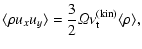 |
(22) |
| |
|
 |
(23) |
Here
 and
and
 are the turbulent
viscosities due to the velocity field and the magnetic field, respectively. We
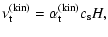
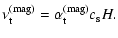
can furthernormalise the turbulent viscosities by the sound speed and gas scale height H (Pringle 1981; Shakura & Sunyaev 1973),
are the turbulent
viscosities due to the velocity field and the magnetic field, respectively. We
can furthernormalise the turbulent viscosities by the sound speed and gas scale height H (Pringle 1981; Shakura & Sunyaev 1973),
| |
|
 |
(24) |
| |
|
 |
(25) |
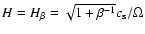
For the gas scale height we use the expression
 ,
with
,
with
 given by the initial value. The resulting -values are given in Table 3. The large scale vertical fields arising from the Parker instability, together with a non-axisymmetric instability in the azimuthal field, give rise to
 ,
resulting in very high accretion rates through
,
resulting in very high accretion rates through
 (Pringle 1981).
Machida et al. (2000) observed similarly high -values in their global simulation of a strongly magnetised accretion disc, and they attributed the Maxwell stresses to a non-axisymmetric magnetorotational instability of the azimuthal field. Kim et al. (2002) considered the competition between Parker and gravitational instabilities in the context of a galactic potential. Simulations including rotation and shear nevertheless did not show any sign of the magnetorotational
instability and the authors note that the magnetorotational instability in the azimuthal field grows too slowly to show up in the simulation time-scale of 4-5 orbits. In this work we find that the onset of turbulence fits a two layer scenario where the atmosphere is dominated by Parker instability and MRI in the ensuing vertical fields, whereas azimuthal field MRI drives the linear growth within a couple of scale heights of the disc midplane.
The kinetic and magnetic energy spectra are shown in Fig. 10
for runs S3D_256 and S3D_512. We have taken the power at scale  ,
,
 ,
and summed over shells of constant wave number
,
and summed over shells of constant wave number
 ,
excluding the anisotropic scale
,
excluding the anisotropic scale
 that is only present in the
y-direction. Figure 10 shows that kinetic energy dominates over
magnetic energy by approximately a factor of two at most scales, except for the
1-2 largest scales which are dominated by the magnetic field.
that is only present in the
y-direction. Figure 10 shows that kinetic energy dominates over
magnetic energy by approximately a factor of two at most scales, except for the
1-2 largest scales which are dominated by the magnetic field.
Table 3:
Turbulent viscosity coefficients and -values, based on
Eqs. (22)-(25).
![\begin{figure}
\par\includegraphics[width=8.1cm,clip]{0385fi10.eps} \end{figure}](/articles/aa/full/2008/41/aa10385-08/Timg239.gif) |
Figure 10:
Kinetic and magnetic energy spectrum for runs S3D_256 and S3D_512.
The power
has been averaged over snapshots between 15 and 20 orbits and summed over
shells of constant wave number
.
Kinetic
energy dominates over magnetic energy at most scales, except for the few
largest scale of the box. |
| Open with DEXTER |
5 Field confinement
![\begin{figure}
\par\includegraphics[width=8.1cm,clip]{0385fi11.eps} \end{figure}](/articles/aa/full/2008/41/aa10385-08/Timg242.gif) |
Figure 11:
Different terms in the azimuthal component of the induction equation
averaged over x and y and over evenly spaced snapshots between
 and
and
 ,
for run S3D_256. The azimuthal
magnetic field is in equilibrium between turbulent transport, representing
compression and advection due to both the mean and the fluctuating velocity
field (turbulent resistivity), and the Keplerian stretching term
that creates By out of Bx. ,
for run S3D_256. The azimuthal
magnetic field is in equilibrium between turbulent transport, representing
compression and advection due to both the mean and the fluctuating velocity
field (turbulent resistivity), and the Keplerian stretching term
that creates By out of Bx. |
| Open with DEXTER |
![\begin{figure}
\par\includegraphics[width=8.3cm,clip]{0385fi12.eps} \end{figure}](/articles/aa/full/2008/41/aa10385-08/Timg243.gif) |
Figure 12:
The radial component of the magnetic field, Bx, averaged over the
radial and azimuthal directions, for runs with Lz=12 H ( top panel) and
Lz=18H ( bottom panel). The vertical structure quickly develops a peak in
the midplane and one additional peak on each side of the midplane, and
this structure stays statistically unchanged for the duration of the
simulation. This radial field creates azimuthal field, by stretching in the Keplerian shear, that balances the
turbulent resistivity acting on the mean azimuthal field (see
Fig. 11). |
| Open with DEXTER |
An important issue related to our proposed path to accretion is whether the
original azimuthal flux can stay confined in the disc or whether it will escape
to infinity by the action of turbulent resistivity (i.e. magnetic buoyancy).
The combination of Parker and interchange instabilities in the non-shearing
frame will eventually redistribute the azimuthal magnetic field evenly over the
entire box height (see Fig. 4). We emphasise that we do not
see the same behaviour in the shearing sheet. The magnetic field and
velocity field stay statistically constant for the entire duration of the
simulations, with no sign of decay or gradual loss of azimuthal flux
(Fig. 7).
5.1 Vertical structure of the field
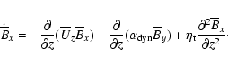
In Fig. 11 we dissect the equilibrium state of By by
averaging different terms from the induction equation over x and y and over
evenly spaced snapshots between
and
.
There
is an almost perfect equilibrium between turbulent transport of magnetic fields
(
 ), representing compression and advection due
to both the mean part of the velocity field and the fluctuating part
(``turbulent resistivity'') and azimuthal field created by the Keplerian shear from the
radial field [
), representing compression and advection due
to both the mean part of the velocity field and the fluctuating part
(``turbulent resistivity'') and azimuthal field created by the Keplerian shear from the
radial field [
 ]. This Keplerian stretching allows for
a closure of the entire process by which strong accretion occurs from initially
purely azimuthal fields. The regular magnetic stretching term
]. This Keplerian stretching allows for
a closure of the entire process by which strong accretion occurs from initially
purely azimuthal fields. The regular magnetic stretching term
 (which does not include stretching by the Keplerian shear because we measure
velocities relative to the main shear) is generally of the same sign as the
turbulent transport term and thus acts oppositely of the Keplerian shear term.
(which does not include stretching by the Keplerian shear because we measure
velocities relative to the main shear) is generally of the same sign as the
turbulent transport term and thus acts oppositely of the Keplerian shear term.
![\begin{figure}
\par\includegraphics[width=8.1cm,clip]{0385fi13.eps} \end{figure}](/articles/aa/full/2008/41/aa10385-08/Timg248.gif) |
Figure 13:
The power contribution to the radially and azimuthally averaged
radial field, as a function of time measured in orbits. Power is provided
almost exclusively by the magnetic stretching term
 ,
while advection and compression are both sink terms. ,
while advection and compression are both sink terms. |
| Open with DEXTER |
The vertical and temporal dependence of the radial magnetic field Bx is
shown in Fig. 12 as a function of height over the midplane z and time t measured in orbits. After around 5 orbits a clear structure evolves out of the flow, with a peak of Bx in the midplane of the disc, followed by a valley and an additional peak at each side of the midplane. This structure stays statistically unchanged for the entire duration of the run. A similar
steady state structure of the radial field was observed by
Hanasz et al. (2002) in rigid rotation simulations of the galactic Parker
instability. In the simulations of Hanasz et al. (2002) Bx would be either
positive or negative in the midplane, depending on the radial wave number of
the initial perturbation. In the shearing sheet the radial wave number of the
PI is forced by the shear to be quite high, and our observation of a positive
radial field in the midplane agrees with the high radial wave number
simulations of Hanasz et al. (2002). Because we include shear in our
simulations we additionally see the constant creation of a z-dependent By,
by the Keplerian shear, which balances out the turbulent transport and prevents
the azimuthal field from spreading evenly over the box height.
In Fig. 13 we show the power contribution to the
large scale Bx as a function of time. We have first averaged Bx and the
advection, compression and stretching terms of the radial component of the
induction equation over the x- and y-directions. The power contribution of
each term is extracted by multiplying the time derivative  with
Bx and averaging over z. Power is provided almost exclusively by the
magnetic stretching term
with
Bx and averaging over z. Power is provided almost exclusively by the
magnetic stretching term
 ,
whereas both
advection and compression extract energy from Bx at all times (except for a
few peaks to around zero power). The magnetic stretching term provides a direct
coupling between Bx and By, indicating that Bx is created from Byin a dynamo process.
,
whereas both
advection and compression extract energy from Bx at all times (except for a
few peaks to around zero power). The magnetic stretching term provides a direct
coupling between Bx and By, indicating that Bx is created from Byin a dynamo process.
![\begin{figure}
\par\includegraphics[width=16.7cm,clip]{0385fi14.eps} \end{figure}](/articles/aa/full/2008/41/aa10385-08/Timg253.gif) |
Figure 14:
Derivation of the dynamo
 from a single snapshot
( top panels) and from the average of several snapshots ( bottom panels). The
(negative) integral of the magnetic stretching term
from a single snapshot
( top panels) and from the average of several snapshots ( bottom panels). The
(negative) integral of the magnetic stretching term
 is shown together with the azimuthal
magnetic field
is shown together with the azimuthal
magnetic field
 ,
both as functions of height over the
midplane, in the left panels. The electromotoric force contribution from
the stretching term is of opposite sign on each side of the midplane. The
right panels show the correlation between
and
,
with orange (grey) denoting points
above the midplane and blue (dark) denoting points below. There is a very
clear correlation (anticorrelation) above (below) the midplane, indicating
a dynamo
that is positive above the midplane and negative below,
and of order ,
both as functions of height over the
midplane, in the left panels. The electromotoric force contribution from
the stretching term is of opposite sign on each side of the midplane. The
right panels show the correlation between
and
,
with orange (grey) denoting points
above the midplane and blue (dark) denoting points below. There is a very
clear correlation (anticorrelation) above (below) the midplane, indicating
a dynamo
that is positive above the midplane and negative below,
and of order
 . . |
| Open with DEXTER |
The creation of a systematic radial field component can be understood from gas
that plunges down field lines that have been bent by the Parker
instability (Parker 1992; Hanasz et al. 2004; Rozyczka et al. 1995; Hanasz & Lesch 1993). As gas slides
azimuthally along the field lines, the Coriolis force causes a counter
clockwise rotation around dense clumps and clockwise rotation around underdense
regions, twisting magnetic field lines in such a way that the perturbed
electromotoric force points parallel to the (unperturbed) azimuthal field
line. Radial field is subsequently created from the stretching of the
perturbed field lines, in much the same way as imagined for the canonical
-mechanism (Parker 1955; Moffatt 1978).
To explore this scenario in more quantitative terms we follow
Moffatt (1978) and expand the velocity and magnetic fields in constant and
fluctuating parts,
 ,
,
 ,
leading to the following evolution equation
for the mean magnetic field
,
leading to the following evolution equation
for the mean magnetic field
 |
(26) |
Here overlines denote azimuthal and radial (and possible temporal) averaging,
while
is a parameter that describes the proportionality
between mean field
 and fluctuating electromotoric force
 .
The parameter
.
The parameter
 represents
turbulent resistivity, proportional to the current density
represents
turbulent resistivity, proportional to the current density
 of the mean field. Writing out
the radial component of Eq. (26) we get
of the mean field. Writing out
the radial component of Eq. (26) we get
 |
(27) |
The first term is due to advection of the large scale radial field by the large
scale vertical velocity component. Figure 13
showed that the source of magnetic energy in the x-component is the magnetic
stretching term. We may thus identify the positive contribution to
 with the properly averaged stretching term,
 |
(28) |
We can subsequently estimate
from
 |
(29) |
by integrating the magnetic stretching term over z. This is of course only a
crude approximation of
that ignores many of the
complications of analysing the evolution of the mean field component (see
e.g. Brandenburg et al. 2008; Brandenburg 2001), but this method gives a good
order of magnitude estimate of the efficiency of creating radial field from the
large scale azimuthal field.
In the left panels of Fig. 14 we plot the integral
as a function of height over the midplane
and compare it to the azimuthal magnetic field
.
The electromotoric force contribution of the magnetic stretching term is of opposite sign at each side of the midplane. The correlation between
and
is shown in
the right panels of Fig. 14, with orange (grey) symbols indicating points above the midplane and blue (dark) symbols indicating points below the midplane. Anticorrelation below the midplane and correlation above indicates a positive
above the midplane and a negative
below the midplane, of the order
for run S3D_256. The higher resolution run S3D_512 gives
 .
The fact that the helicity dynamo increases in efficiency when going to higher resolution, even though both the collisional hyper and shock resistivity coefficients are reduced, may indicate that the outlined dynamo is a fast dynamo, although future simulations applying resistivity on physical rather than on numerical grounds will be needed to
corroborate this point (see e.g. Hanasz et al. 2002).
.
The fact that the helicity dynamo increases in efficiency when going to higher resolution, even though both the collisional hyper and shock resistivity coefficients are reduced, may indicate that the outlined dynamo is a fast dynamo, although future simulations applying resistivity on physical rather than on numerical grounds will be needed to
corroborate this point (see e.g. Hanasz et al. 2002).
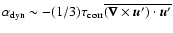
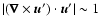
Considering the creation of radial field by the Parker instability in a
galactic environment, Hanasz & Lesch (1993) predict
 ,
where the ``cyclonic velocity''
,
where the ``cyclonic velocity''
 of
Parker (1979) is approximately
of
Parker (1979) is approximately
 in our simulations. The
resulting dynamo coefficient
in our simulations. The
resulting dynamo coefficient
 is quite
similar to what we find here from integrating the magnetic stretching term. In
the theoretical framework of Moffatt (1978), on the other hand, the value
of
should be comparable to the correlation time of the
turbulence
is quite
similar to what we find here from integrating the magnetic stretching term. In
the theoretical framework of Moffatt (1978), on the other hand, the value
of
should be comparable to the correlation time of the
turbulence
 times the mean helicity,
 ,
at
least in the limit of vanishing collisional resistivity. The helicity in our
simulations is positive below the midplane and negative above the midplane,
with an amplitude of
,
at
least in the limit of vanishing collisional resistivity. The helicity in our
simulations is positive below the midplane and negative above the midplane,
with an amplitude of
 .
Thus the
inferred sign of
fits well with the analytical theory, but
the absolute value of
is at least ten times smaller than the
expectation based on a correlation time of order unity. This discrepancy may be
simply due to the fact that kinematic dynamo theory is not applicable to our
simulations, because the Lorentz force plays a significant role in determining
the evolution of the velocity field and the magnetic field.
.
Thus the
inferred sign of
fits well with the analytical theory, but
the absolute value of
is at least ten times smaller than the
expectation based on a correlation time of order unity. This discrepancy may be
simply due to the fact that kinematic dynamo theory is not applicable to our
simulations, because the Lorentz force plays a significant role in determining
the evolution of the velocity field and the magnetic field.
6 Summary and conclusions
In this paper we consider the evolution of strongly magnetised Keplerian
accretion discs. Our numerical experiments show that the hydromagnetic state of
the gas flow is very different from what is seen in zero net flux simulations.
The Parker instability leads to huge magnetic arcs rising several scale heights
from the disc midplane, and the magnetorotational instability in turn feeds
off the vertical fields and creates a highly turbulent flow, an interaction
that was predicted analytically by Tout & Pringle (1992). Although the flow is
stochastic and time fluctuating, we have identified an underlying dynamo
process that couples the vertically dependent mean radial and azimuthal
magnetic field components. As gas slides down inclined field lines, it obtains
a helical motion due to Coriolis forces, and thus the azimuthal field lines are
twisted in such a way as to create a mean electromotoric force in the direction
of the unperturbed field line - a configuration prone to create radial field.
In turn the large scale radial field regenerates the azimuthal field through stretching in the
Keplerian shear. Although Parker instability dominates the linear growth
phase, we have found evidence for magnerotational instability in the azimuthal
field as well. In the midplane of the disc, where the buoyancy is weak,
azimuthal MRI drives the initial evolution towards turbulence
(Foglizzo & Tagger 1995,1994; Terquem & Papaloizou 1996). These two
related instabilities, magnetorotational instability in the vertical fields
created by the Parker instability and magnetorotational swing instability in
the azimuthal fields, both rely on azimuthal flux confinement and can coexist in
the linear as well as in the non-linear state of transmagnetic accretion discs.
Such a path to accretion, based on the interaction of Parker and
magnetorotational instabilities, has at least two appealing traits. First of
all that the vertical fields that feed the magnetorotational instability are
created in a transparent way by the Parker instability. Zero magnetic flux
models must most likely rely on a small scale dynamo in order to create
vertical fields, and there is mounting evidence that such a dynamo would not
operate in the bulk part of accretion discs where the magnetic Prandtl number
is much lower than unity (Schekochihin et al. 2005; Fromang et al. 2007).
The second appealing result of our model is that the Maxwell and Reynolds
stresses are significant (
 ). Such high accretion stresses
could solve the problem that observed accretion rates are often one or two
orders of magnitude higher than the accretion rates obtained in zero net flux
MRI simulations (King et al. 2007).
). Such high accretion stresses
could solve the problem that observed accretion rates are often one or two
orders of magnitude higher than the accretion rates obtained in zero net flux
MRI simulations (King et al. 2007).
The regeneration of azimuthal field by the shearing of an appropriate radial
field was seen in all our simulations that included Keplerian shear. As
magnetohydrostatic equilibrium is compromised by the Parker instability, gas
streams down along inclined field lines. Coriolis force diverts the gas to the
right, and a radial magnetic field is created as the azimuthal field is
subjected to shear-regions typically the size of the Parker instability.
Eventually magnetic reconnection leads to a coherent large scale radial
magnetic field. This dynamo was predicted by Parker (1992) and subsequently
observed in the rigid rotation simulations of Hanasz et al. (2002). To our
knowledge we are the first to point out the relevance of Parker's fast galactic
dynamo to accretion discs and how it closes the accretion loop by replenishing
the azimuthal field that is lost by magnetic buoyancy.
The fine-tuned initial conditions with a purely azimuthal magnetic field and a
constant ratio of magnetic to thermal pressure may be questioned. However our
experiments with a combined azimuthal and vertical field shows that the Parker
instability is robust even if the azimuthal field coexists with a moderately
strong net vertical field, and that the additional vertical field component may
indeed increase the accretion rate further.
Our results may also be relevant for star formation in the galactic centre.
Although there is currently no coherent accretion disc structure, the
population of young, massive stars in a disc-like structure close to the
galactic centre points towards the brief existence of an accretion disc some
million years ago
(Levin & Beloborodov 2003; Nayakshin et al. 2007; Alexander et al. 2008; Milosavljevic & Loeb 2004).
The disc was likely to be initially strongly magnetised, as indicated by the
current high magnetisation of the circumnuclear molecular ring. Hence the type
of MHD processes studied in this paper may be of central significance for the
disc dynamics. The presented simulations of transmagnetic (
 )
discs
argues that discs dominated by magnetic pressure
)
discs
argues that discs dominated by magnetic pressure
 are
astrophysically viable. The existence of such discs was conjectured by
Pariev et al. (2003) and their limitations and observational consequences
were explored by Begelman & Pringle (2007). A number of problems in accretion
disc theory are alleviated by the presence of super-equipartition magnetic
fields, among them is the long-standing issue of self-gravity and fragmentation
of AGN discs (Goodman 2003).
are
astrophysically viable. The existence of such discs was conjectured by
Pariev et al. (2003) and their limitations and observational consequences
were explored by Begelman & Pringle (2007). A number of problems in accretion
disc theory are alleviated by the presence of super-equipartition magnetic
fields, among them is the long-standing issue of self-gravity and fragmentation
of AGN discs (Goodman 2003).
Future research into strongly magnetised accretion discs should also focus on
the self-consistent modelling of the
magnetisation of the material that feeds accretion discs in various
environments and on the evolution of magnetised disc coronae, in light of
effects such as reconnection, shearing of foot points, Ohmic heating and
radiative cooling that take place there.
Acknowledgements
Computer simulations were performed at the PIA cluster of the Max Planck
Institute for Astronomy and at the SARA Computing and Networking Service in
Amsterdam. We would like to thank Micha Hanasz, Steve Balbus, and Andrew
King for inspiring discussions. Axel Brandenburg, Jim Pringle and Richard
Alexander are thanked for commenting an early version of the manuscript.
We are grateful to Gordon Ogilvie and to the referee, Thierry Foglizzo,
for pointing out the relevance of the azimuthal field MRI for our simulations.
Hanasz, Steve Balbus, and Andrew
King for inspiring discussions. Axel Brandenburg, Jim Pringle and Richard
Alexander are thanked for commenting an early version of the manuscript.
We are grateful to Gordon Ogilvie and to the referee, Thierry Foglizzo,
for pointing out the relevance of the azimuthal field MRI for our simulations.
- Alexander, R. D.,
Armitage, P. J., Cuadra, J., & Begelman, M. C. 2008,
ApJ, 674, 927 [NASA ADS] [CrossRef]
-
Balbus, S. A., & Hawley, J. F. 1991, ApJ, 376,
21 [NASA ADS] [CrossRef]
(In the text)
-
Balbus, S. A., & Hawley, J. F. 1992, ApJ, 400,
610 [NASA ADS] [CrossRef]
-
Balbus, S. A., & Henri, P. 2008, ApJ, 674, 408 [NASA ADS] [CrossRef]
(In the text)
- Basu, S., Mouschovias,
T. C., & Paleologou, E. V. 1997, ApJ, 480, L55 [NASA ADS] [CrossRef]
(In the text)
- Begelman, M. C., &
Pringle, J. E. 2007, MNRAS, 375, 1070 [NASA ADS] [CrossRef]
(In the text)
- Blaes, O., Hirose, S.,
& Krolik, J. H. 2007, ApJ, 664, 1057 [NASA ADS] [CrossRef]
(In the text)
-
Brandenburg, A. 2001, ApJ, 550, 824 [NASA ADS] [CrossRef]
-
Brandenburg, A. 2003, in Advances in nonlinear dynamos, ed. A.
Ferriz-Mas, & M. Núñez (London and New York: Taylor
& Francis), The Fluid Mech. of Astrophys. Geophys., 9, 269
(In the text)
- Brandenburg, A., &
Subramanian, K. 2005, Phys. Rep., 417, 1 [NASA ADS] [CrossRef]
(In the text)
- Brandenburg, A.,
Nordlund, Å., Stein, R. F., & Torkelsson, U. 1995, ApJ,
446, 741 [NASA ADS] [CrossRef]
- Brandenburg, A.,
Rädler, K.-H., Rheinhardt, M., & Käpylä,
P. J. 2008, ApJ, 676, 740 [NASA ADS] [CrossRef]
- Dobler, W., Stix, M.,
& Brandenburg, A. 2006, ApJ, 638, 336 [NASA ADS] [CrossRef]
(In the text)
-
Foglizzo, T., & Tagger, M. 1994, A&A, 287, 297 [NASA ADS]
-
Foglizzo, T., & Tagger, M. 1995, A&A, 301, 293 [NASA ADS]
-
Fromang, S., & Nelson, R. P. 2006, A&A, 457, 343 [NASA ADS] [CrossRef] [EDP Sciences]
- Fromang, S., & Papaloizou,
J. 2007, A&A, 476, 1113 [NASA ADS] [CrossRef] [EDP Sciences]
- Fromang, S., Papaloizou,
J., Lesur, G., & Heinemann, T. 2007, A&A, 476, 1123 [NASA ADS] [CrossRef] [EDP Sciences]
- Goodman,
J. 2003, MNRAS, 339, 937 [NASA ADS] [CrossRef]
(In the text)
-
Greenhill, L. J. 2007, in IAU Symp., 242, 381
-
Hanasz, M., & Lesch, H. 1993, A&A, 278, 561 [NASA ADS]
- Hanasz, M.,
Otmianowska-Mazur, K., & Lesch, H. 2002, A&A, 386, 347 [NASA ADS] [CrossRef] [EDP Sciences]
(In the text)
- Hanasz, M., Kowal, G.,
Otmianowska-Mazur, K., & Lesch, H. 2004, ApJ, 605, L33 [NASA ADS] [CrossRef]
- Haugen,
N. E. L., Brandenburg, A., & Mee, A. J. 2004,
MNRAS, 353, 94 [NASA ADS] [CrossRef]
(In the text)
- Hawley, J. F.,
Gammie, C. F., & Balbus, S. A. 1996, ApJ, 464,
690 [NASA ADS] [CrossRef]
- Heinemann, T.,
Nordlund, Å., Scharmer, G. B., & Spruit, H. C.
2007, ApJ, 669, 1390 [NASA ADS] [CrossRef]
(In the text)
- Hildebrand,
R. H., Gonatas, D. P., Platt, S. R., et al.
1990, ApJ, 362, 114 [NASA ADS] [CrossRef]
-
Johansen, A., & Klahr, H. 2005, ApJ, 634, 1353 [NASA ADS] [CrossRef]
- Keppens, R., Casse, F.,
& Goedbloed, J. P. 2002, ApJ, 569, L121 [NASA ADS] [CrossRef]
- Kim, J., Hong, S. S.,
& Ryu, D. 1997, ApJ, 485, 228 [NASA ADS] [CrossRef]
- Kim, J., Hong, S. S.,
Ryu, D., & Jones, T. W. 1998, ApJ, 506, L139 [NASA ADS] [CrossRef]
(In the text)
- Kim, W.-T., Ostriker,
E. C., & Stone, J. M. 2002, ApJ, 581, 1080 [NASA ADS] [CrossRef]
(In the text)
- King, A. R., Pringle,
J. E., & Livio, M. 2007, MNRAS, 376, 1740 [NASA ADS] [CrossRef]
(In the text)
- Lesur, G., & Longaretti, P.-Y.
2007, MNRAS, 378, 1471 [NASA ADS] [CrossRef]
-
Lesur, G., & Ogilvie, G. I. 2008, A&A, 488, 451 [NASA ADS] [CrossRef] [EDP Sciences]
- Levin, Y., & Beloborodov,
A. M. 2003, ApJ, 590, L33 [NASA ADS] [CrossRef]
- Machida, M., Hayashi,
M. R., & Matsumoto, R. 2000, ApJ, 532, L67 [NASA ADS] [CrossRef]
(In the text)
- Matsumoto, R., Tajima,
T., Shibata, K., & Kaisig, M. 1993, ApJ, 414, 357 [NASA ADS] [CrossRef]
(In the text)
-
Miller, K. A., & Stone, J. M. 2000, ApJ, 534,
398 [NASA ADS] [CrossRef]
(In the text)
- Milosavljevic, M., & Loeb,
A. 2004, ApJ, 604, L45 [NASA ADS] [CrossRef]
- Moffatt,
H. K. 1978, Magnetic field generation in electrically
conducting fluids (Cambridge, England: Cambridge University
Press)
-
Mouschovias, T. C. 1974, ApJ, 192, 37 [NASA ADS] [CrossRef]
(In the text)
- Nayakshin, S., Cuadra,
J., & Springel, V. 2007, MNRAS, 379, 21 [NASA ADS] [CrossRef]
- Pariev, V. I.,
Blackman, E. G., & Boldyrev, S. A. 2003, A&A,
407, 403 [NASA ADS] [CrossRef] [EDP Sciences]
(In the text)
- Parker,
E. N. 1955, ApJ, 122, 293 [NASA ADS] [CrossRef]
- Parker,
E. N. 1966, ApJ, 145, 811 [NASA ADS] [CrossRef]
(In the text)
- Parker,
E. N. 1979, Cosmical magnetic fields: Their origin and their
activity (Oxford: Clarendon Press; New York: Oxford University
Press)
(In the text)
- Parker,
E. N. 1992, ApJ, 401, 137 [NASA ADS] [CrossRef]
- Pessah, M. E., Chan,
C., & Psaltis, D. 2007, ApJ, 668, 51 [NASA ADS] [CrossRef]
(In the text)
- Pringle,
J. E. 1981, ARA&A, 19, 137 [NASA ADS] [CrossRef]
-
Regev, O., & Umurhan, O. M. 2008, A&A, 481, 21 [NASA ADS] [CrossRef] [EDP Sciences]
- Rincon, F., Ogilvie,
G. I., & Proctor, M. R. E. 2007, Phys. Rev.
Lett., 98, 254502 [NASA ADS] [CrossRef]
- Rozyczka,
M., Joung Turner, N., & Bodenheimer, P. 1995, MNRAS, 276,
1179 [NASA ADS]
- Sano, T., Inutsuka, S.-I.,
Turner, N. J., & Stone, J. M. 2004, ApJ, 605,
321 [NASA ADS] [CrossRef]
- Schekochihin,
A. A., Haugen, N. E. L., Brandenburg, A.,
et al. 2005, ApJ, 625, L115 [NASA ADS] [CrossRef]
(In the text)
-
Shakura, N. I., & Sunyaev, R. A. 1973, A&A, 24,
337 [NASA ADS]
- Shu, F. H. 1974,
A&A, 33, 55 [NASA ADS]
(In the text)
- Terquem, C., & Papaloizou,
J. C. B. 1996, MNRAS, 279, 767 [NASA ADS]
- Tout,
C. A., & Pringle, J. E. 1992, MNRAS, 259, 604 [NASA ADS]
(In the text)
- Vlemmings,
W. H. T., Bignall, H. E., & Diamond, P. J.
2007, ApJ, 656, 198 [NASA ADS] [CrossRef]
-
Wardle, M., & Konigl, A. 1990, ApJ, 362, 120 [NASA ADS] [CrossRef]
Copyright ESO 2008
![$\displaystyle \frac{B_y^2}{2\mu_0} = \beta^{-1} c_{\rm s}^2 \rho_0 \exp[-z^2/(2
H_\beta^2)],$](/articles/aa/full/2008/41/aa10385-08/img96.gif)
![$\displaystyle A_x(z) = \sqrt{2 \pi \mu_0 \beta^{-1} c_{\rm s}^2 \rho_0}
H_\beta {\rm erf}[z/(2 H_\beta)].$](/articles/aa/full/2008/41/aa10385-08/img97.gif)
![\begin{figure}
\par\includegraphics[width=8.4cm,clip]{0385fi1a.eps}\hspace*{2mm}...
....eps}\hspace*{2mm}
\includegraphics[width=8.4cm,clip]{0385fi1d.eps}\end{figure}](/articles/aa/full/2008/41/aa10385-08/img107.gif)
![\begin{figure}
\par\includegraphics[width=8.2cm,clip]{0385fig2.eps} \end{figure}](/articles/aa/full/2008/41/aa10385-08/img114.gif)
![\begin{figure}
\par\includegraphics[width=8.2cm,clip]{0385fig3.eps} \end{figure}](/articles/aa/full/2008/41/aa10385-08/img115.gif)
![\begin{figure}
\par\includegraphics[width=8.2cm,clip]{0385fig4.eps} \end{figure}](/articles/aa/full/2008/41/aa10385-08/img116.gif)
![\begin{figure}
\par\mbox{\includegraphics[width=1.5cm]{0385fi5a.eps} \includegra...
...1.5cm]{0385fi5g.eps} \includegraphics[width=8.8cm]{0385fi5h.eps} }
\end{figure}](/articles/aa/full/2008/41/aa10385-08/img117.gif)
![\begin{figure}
\par\includegraphics[width=7cm,clip]{0385fig6.eps} \end{figure}](/articles/aa/full/2008/41/aa10385-08/img123.gif)
![\begin{figure}
\par\includegraphics[width=8.2cm,clip]{0385fig7.eps} \end{figure}](/articles/aa/full/2008/41/aa10385-08/img125.gif)
![\begin{figure}
\par\includegraphics[width=8.1cm,clip]{0385fig8.eps} \end{figure}](/articles/aa/full/2008/41/aa10385-08/img133.gif)
![\begin{figure}
\par\includegraphics[width=8.2cm,clip]{0385fig9.eps} \end{figure}](/articles/aa/full/2008/41/aa10385-08/img220.gif)
![\begin{figure}
\par\includegraphics[width=8.1cm,clip]{0385fi10.eps} \end{figure}](/articles/aa/full/2008/41/aa10385-08/img239.gif)
![\begin{figure}
\par\includegraphics[width=8.1cm,clip]{0385fi11.eps} \end{figure}](/articles/aa/full/2008/41/aa10385-08/img242.gif)
![\begin{figure}
\par\includegraphics[width=8.3cm,clip]{0385fi12.eps} \end{figure}](/articles/aa/full/2008/41/aa10385-08/img243.gif)
![\begin{figure}
\par\includegraphics[width=8.1cm,clip]{0385fi13.eps} \end{figure}](/articles/aa/full/2008/41/aa10385-08/img248.gif)
![\begin{figure}
\par\includegraphics[width=16.7cm,clip]{0385fi14.eps} \end{figure}](/articles/aa/full/2008/41/aa10385-08/img253.gif)