A&A 490, 477-486 (2008)
DOI: 10.1051/0004-6361:200809682
A new equation for the mid-plane potential of power law discs
II. Exact solutions and approximate formulae
J.-M. Huré1,2 - F. Hersant2 - C. Carreau3 - J.-P. Busset1
1 - Université de Bordeaux, LAB, 351 cours de la Libération, Talence 33405, France
2 -
CNRS/INSU, UMR 5804/LAB, 2 rue de l'Observatoire, BP 89, 33271 Floirac Cedex, France
3 -
La Maurellerie, 37290 Bossay-sur-Claise, France
Received 29 February 2008 / Accepted 31 May 2008
Abstract
Aims. The first-order ordinary differential equation (ODE) that describes the mid-plane gravitational potential in flat finite size discs of surface density
 (Huré & Hersant 2007, A&A, 467, 907) is solved exactly in terms of infinite series.
Methods. The formal solution of the ODE is derived and then converted into a series representation by expanding the elliptic integral of the first kind over its modulus before analytical integration.
Results. Inside the disc, the gravitational potential consists of three terms: a power law of radius R with index 1+s, and two infinite series of the variables R and 1/R. The convergence of the series can be accelerated, enabling the construction of reliable approximations. At the lowest-order, the potential inside large astrophysical discs (
 )
is described by a very simple formula whose accuracy (a few percent typically) is easily increased by considering successive orders through a recurrence. A basic algorithm is given.
)
is described by a very simple formula whose accuracy (a few percent typically) is easily increased by considering successive orders through a recurrence. A basic algorithm is given.
Conclusions. Applications concern all theoretical models and numerical simulations where the influence of disc gravity must be checked and/or reliably taken into account.
Key words: gravitation - methods: analytical - accretion, accretion disks
Gaseous discs in which the main physical quantities (density, pressure, temperature, thickness, velocity) scale with cylindrical radius as power laws, i.e. ``power-law discs'', represent an important class of theoretical systems. These are used customary to model accretion in evolved binaries (Shakura & Sunyaev 1973; Pringle 1981), circumstellar matter (Edgar 2007; Dubrulle 1992), the environment of massive black holes inside active galactic nuclei (Collin-Souffrin & Dumont 1990; Huré 1998; Semerák 2004) or even the stellar component of some galaxies (Evans 1994; Zhao et al. 1999). In most applications however, power-law discs are truncated either to avoid diverging values at the disc centre (such as density, mass) or in attempting to reproduce the properties of observed discs of finite extension and mass. Although self-similarity is not compatible with the presence of edges, it is generally considered that power laws offer a good description of disc properties in some regions (far from the edges). Note that the presence of sharp edges can be misleading when interpreting observational data (e.g. Hughes et al. 2008). In general, the surface density  in the outer parts of discs is a decreasing function of the cylindrical radius R. Depending on the models, hypotheses, and objects, we have, for instance,
 in binaries (Shakura & Sunyaev 1973),
 in active galactic nuclei (Collin-Souffrin & Dumont 1990),
 for a Mestel disc (Mestel 1963), or
 in circumstellar discs (Piétu et al. 2007). In the context of stationary viscous
  -discs, a wide range of power-law exponents is allowed since the temperature T, ,
and R satisfy the condition (e.g. Pringle 1981):
-discs, a wide range of power-law exponents is allowed since the temperature T, ,
and R satisfy the condition (e.g. Pringle 1981):
while it is
 in
in  -discs (Huré et al. 2001).
The calculus of the gravitation potential of finite-size, power-law discs has received little attention yet. Several reasons can be put forward. Solving the Poisson equation or computing the integral of the potential is not a trivial procedure, especially in the presence of edges. It is generally believed that gravity due to low mass discs is unimportant compared with that of a central proto-star or black hole, and cannot be probed (see however Baruteau & Masset 2008). Many studies employ the multi-pole expansion which is known to converge too slowly inside sources to be efficient for the numerical applications (e.g. Stone & Norman 1992; Clement 1974). Huré & Hersant (2007) demonstrated that the mid-plane potential of flat power-law discs obeys an inhomogeneous first-order ordinary differential equation (ODE). In this second paper, we discuss the exact solutions of this ODE for the entire physical range (outside and inside the disc) in terms of infinite series. In particular, it is shown that the mid-plane potential is a combination of a power law for the radius R and two series of the variables R and 1/R. Since these series converge rapidly inside large discs, it is possible to derive reliable approximations by truncating the series at low orders.
This paper is organised as follows. The ODE for the potential is briefly recalled in Sect. 2 and its formal solution is derived in Sect. 3. In Sect. 4, we express the potential at the two disc edges and consider a few special cases. The inside and outside solutions in the form of series are presented in Sect. 5. In Sect. 6, we analyse the potential in the disc inside in detail, and in particular, the power-law contribution. Since all series involved converge rapidly, we are able to derive reliable approximations for the potential; this is done in Sect. 7. We discuss in Sect. 8 the case of discs with no inner and/or outer edge. The paper ends with a few concluding remarks.
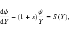
2 The mid-plane potential in power-law discs from an ordinary differential equation (ODE)
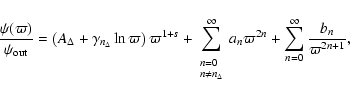
Following Huré & Hersant (2007) hereafter Paper I), the mid-plane potential  due to a flat power-law disc satisfies the ODE:
 |
(1) |
where
 is the cylindrical radius in units of the radius
 of the disc outer edge, s is the power-law index of the surface density ,
namely (generally, s < 0 in astrophysical discs):
of the disc outer edge, s is the power-law index of the surface density ,
namely (generally, s < 0 in astrophysical discs):
 |
(2) |
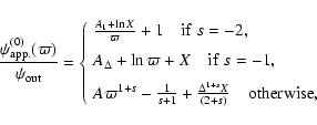
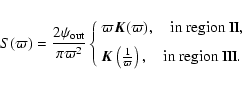
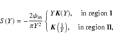
and  is the piecewise defined function. Depending on the position in the disc (see Fig. 1), we have:
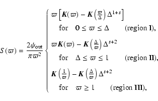 |
(3) |
where
 is the axis ratio,
 is the radius of the inner edge,
 is a positive constant,
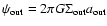
 is the surface density at the disc outer edge,
  is the complete elliptic integral of the first kind:
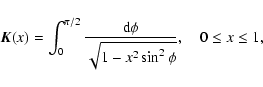 |
(4) |
and G is the gravitation constant. The above ODE can in principle be solved in the entire radial domain since boundary conditions (both
and the associated acceleration
 )
are known precisely at
)
are known precisely at  and at
 for power law distributions. Although S is singular at the two disc edges (i.e. for
 ), Eq. (1) is far more tractable in computing
than the integral form (e.g. Durand 1953):
), Eq. (1) is far more tractable in computing
than the integral form (e.g. Durand 1953):
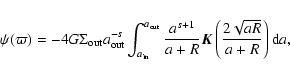 |
(5) |
whose integrand is logarithmically singular everywhere inside the disc, or than the Poisson equation, which involves vertical gradients.
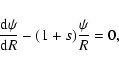
3 Formal solution of the ODE
A formal solution of Eq. (1) is found by setting (e.g. Rybicki & Lightman 1979):
 |
(6) |
and
 |
(7) |
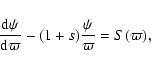
The exact derivative of
 is:
is:
![\begin{displaymath}%
\frac{{\rm d} \bar{\psi}}{{\rm d} \varpi} = \varpi^{-(1+s)}...
...\rm d} \psi}{{\rm d} \varpi} - (1+s)\frac{\psi}{\varpi}\right]
\end{displaymath}](/articles/aa/full/2008/41/aa09682-08/img44.gif) |
(8) |
where we recognise, inside brackets, the function S. Therefore, we have:
 |
(9) |
whose formal solution for
is of the form:
 |
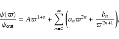
(10) |
Back-substituting
and  from Eqs. (6) and (7), we find the general expression for the mid-plane potential:
![\begin{displaymath}%
\psi(\varpi) = \varpi^{1+s} \left[ \frac{\psi(\varpi_0)}{\v...
...rpi{\frac{S(\varpi')}{{\varpi'}^{1+s}}{\rm d}\varpi'} \right].
\end{displaymath}](/articles/aa/full/2008/41/aa09682-08/img48.gif) |
(11) |
This solution is fully determined in the entire spatial domain or part of it as soon as the potential is known at a given normalised radius  .
We observe that, for
.
We observe that, for  ,
,
 is the mixture of a power law of the radius (the first term in the right-hand-side) with exponent (e.g. Bisnovatyi-Kogan 1975; Evans & Read 1998):
and a complicated function of the radius R (the definite integral).
In the following, we shall analyse Eq. (11) analytically in terms of infinite series by considering in Eq. (3) the expansion of
over its modulus (e.g. Gradshteyn & Ryzhik 1965):
 |
(13) |
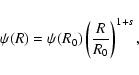
4 Potential at the disc edges
To determine
from Eq. (11) for
 ,
it is sufficient to calculate the potential at the two disc edges
,
it is sufficient to calculate the potential at the two disc edges![[*]](/icons/foot_motif.gif) , that is
, that is
 and
and  .
For this purpose, we use Eq. (5) and define
.
For this purpose, we use Eq. (5) and define
 .
After some algebra we find:
.
After some algebra we find:
 |
(15) |
From Eq. (13), the potential at the inner edge is:
 |
(16) |
where
 |
(17) |
and assuming
 (see below). As
 1/n for large n (see Fig. 2),
consists of terms that vary asymptotically like
1/n for large n (see Fig. 2),
consists of terms that vary asymptotically like  1/n2. Since
 ,
is a converging series.
,
is a converging series.
![\begin{figure}
\par\includegraphics[width=9cm,clip]{fig2hure09682.eps}\end{figure}](/articles/aa/full/2008/41/aa09682-08/Timg65.gif) |
Figure 2:
Coefficient  versus n. Terms an and |dn| versus n for s=-1.5.
 |
| Open with DEXTER |
At the outer edge, the potential is calculated in a similar manner, but using the variable
 .
For
.
For  ,
Eq. (5) writes1:
,
Eq. (5) writes1:
 |
(18) |
Replacing
 by its series representation yields:
 |
(19) |
where
 |
(20) |
and by assuming
(see below). As for
and for the same reasons,
is also a converging series.
4.3 Special values of s
If the power law exponent s is such that:
at a certain rank
 ,
then
must be, in practice, written in a slightly different form. This happens for
,
then
must be, in practice, written in a slightly different form. This happens for
 with:
with:
 |
(22) |
Since
 |
(23) |
for x >0 and any q, we have:
 |
(24) |
Then, if
,
the potential at the disc inner edge is given by:
![\begin{displaymath}
%
\psi(\Delta) = -\psi_{\rm out} \Delta^{1+s} \left[
\sum_{...
...Delta^{2n-s-1}\right)} - \gamma_{n_\Delta} \ln \Delta \right].
\end{displaymath}](/articles/aa/full/2008/41/aa09682-08/img77.gif) |
(25) |
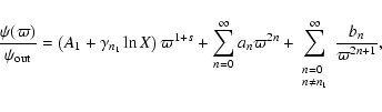
In a similar way, if s is such that:
at a rank
 ,
then one term in Eq. (19) must be treated separately. This happens for
,
then one term in Eq. (19) must be treated separately. This happens for
 where:
 |
(27) |
From Eq. (23), we have:
![\begin{displaymath}%
\psi(1) = -\psi_{\rm out}\left[ \sum_{\begin{array}{l}
{\sc...
...t(1-\Delta^{2n+s+2}\right) - \gamma_{n_1} \ln \Delta} \right].
\end{displaymath}](/articles/aa/full/2008/41/aa09682-08/img81.gif) |
(28) |
We note that s cannot belong simultaneously to set
 and to set
 .
.
The case  occurs i) when the disc has no inner hole (i.e.
 )
but finite size, and/or ii) when the disc has an inner edge but is infinitely extended (i.e.
)
but finite size, and/or ii) when the disc has an inner edge but is infinitely extended (i.e.
 ). In the first case,
(denoted
). In the first case,
(denoted
 in Paper I) becomes the potential at the origin of coordinates and has infinite value as soon as
  .
In the second case,
represents the gravitational potential at infinity. It diverges if
.
In the second case,
represents the gravitational potential at infinity. It diverges if  .
Figure 3 summarises the ranges of s where the edge surface density, edge potential, and total disc mass are finite. We note that only discs having either i)
,
.
Figure 3 summarises the ranges of s where the edge surface density, edge potential, and total disc mass are finite. We note that only discs having either i)
,
 with s > 0; or ii)
 ,
with
,
with  are physically meaningful since they are characterised by a finite surface density, a finite total mass and a finite potential. Mestel discs do not belong to these categories (e.g. Hunter et al. 1984; Mestel 1963).
![\begin{figure}
\par\includegraphics[width=9cm,clip]{fig3hure09682.eps}
\end{figure}](/articles/aa/full/2008/41/aa09682-08/Timg92.gif) |
Figure 3:
Ranges of s where the edge surface density, edge potential and total disc mass are infinite. |
| Open with DEXTER |
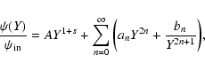
5 Solution of the ODE in the form of series
We see from Eqs. (3) and (13) that the function S can be easily expressed as a series. We have:
 |
(29) |
By inserting this general expression into Eq. (11), we find for
 and
:
and
:
![$\displaystyle %
\psi(\varpi) = \frac{\psi(\varpi_0)}{\varpi_0^{1+s}} \varpi^{1+...
...rac{1}{\varpi^{2n+1}} - \frac{\varpi^{1+s}}{\varpi_0^{2n+2+s}} \right) \right],$](/articles/aa/full/2008/41/aa09682-08/img95.gif) |
|
|
(30) |
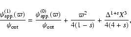
where the coefficients an and bn are respectively given by:
![\begin{displaymath}%
a_n = I_n \times \left \{
\begin{array}{l}
1-\Delta^{1+s-2n...
...~II},\\ [2mm]
0 \quad {\rm in~region~III},
\end{array}\right.
\end{displaymath}](/articles/aa/full/2008/41/aa09682-08/img96.gif) |
(31) |
and
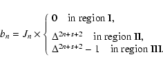 |
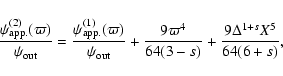
(32) |
Since
and
are available (see Sect. 4), we use
 and
and
 to simplify Eq. (30). Using Eqs. (16) and (19), we thus have:
 |
(33) |
where:
![\begin{displaymath}%
A =\left \{
\begin{array}{l}
0,\quad {\rm in~region~I},\\ [...
...n~II},\\ [2mm]
0,\quad {\rm in~region~III},
\end{array}\right.
\end{displaymath}](/articles/aa/full/2008/41/aa09682-08/img101.gif) |
(34) |
with:
We note that A is a function of s.
Figure 4 compares the total potential
with the power law contribution (i.e. the term
 )
for three typical values of the exponent s in a disc of axis ratio
)
for three typical values of the exponent s in a disc of axis ratio
 .
We clearly see that, in a finite size disc: i) the gravitational potential is not a power-law function of the radius; ii) a power-law contribution is present inside the disc only; and iii) the power law is not the dominant part of the potential. As expected, spatial self-similarity is broken due to edges. We note that, outside the disc (i.e. in regions I and III), the series coincides with the multi-pole expansions.
.
We clearly see that, in a finite size disc: i) the gravitational potential is not a power-law function of the radius; ii) a power-law contribution is present inside the disc only; and iii) the power law is not the dominant part of the potential. As expected, spatial self-similarity is broken due to edges. We note that, outside the disc (i.e. in regions I and III), the series coincides with the multi-pole expansions.
![\begin{figure}
\par\includegraphics[width=9cm,clip]{fig4hure09682.eps}
\end{figure}](/articles/aa/full/2008/41/aa09682-08/Timg102.gif) |
Figure 4:
Potential ( plain lines) in a power-law disc with axis ratio
and
 .
The contribution of the power law, i.e. the term
in Eq. (33), is shown in comparison. .
The contribution of the power law, i.e. the term
in Eq. (33), is shown in comparison. |
| Open with DEXTER |
6 Potential inside the disc
The determination of the gravitational potential is usually straightforward outside the distribution where different kinds of expansions are efficient in practice (Kellogg 1929). In contrast, it is problematic inside matter where the classical multi-pole approach fails to converge rapidly (e.g. Stone & Norman 1992; Clement 1974).
In region II, we have
 .
If we set:
.
If we set:
 |
(36) |
then
 |
(37) |
Figure 2 shows the term an versus n for s=-1.5 (in this case, In=Jn). As a consequence, the three series involved in Eq. (33) converge rapidly since i) In and Jn both vary as 1/n2 at large n; ii) all terms are positive for large n; and iii)
 and
and  .
This is interesting for the truncation of series and the construction of reliable approximations (see Sect. 7).
.
This is interesting for the truncation of series and the construction of reliable approximations (see Sect. 7).
The coefficient A is plotted in Fig. 5. It is symmetric with respect to
 since:
 |
(38) |
where
 .
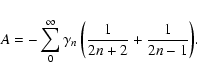
For certain integer values of |s|, A is strictly zero. This is in particular the case for s=-3 and s=0 (see Appendix A). As Eq. (34) shows, A rises as soon as the exponent s is such that either 2n-s-1 or 2n+s+2 is small (see Sect. 4). Even, if
.
For certain integer values of |s|, A is strictly zero. This is in particular the case for s=-3 and s=0 (see Appendix A). As Eq. (34) shows, A rises as soon as the exponent s is such that either 2n-s-1 or 2n+s+2 is small (see Sect. 4). Even, if
 (or n=n1), the coefficient A apparently contains a singular term, namely
 (resp.
 ); however, this singularity exactly cancels with the term
 (resp.
 ). In practice, when
,
Eq. (33) is no longer valid. Instead, we have:
). In practice, when
,
Eq. (33) is no longer valid. Instead, we have:
 |
(39) |
where
 |
(40) |
Similarly, if
,
the potential writes
 |
(41) |
where
![\begin{displaymath}%
A_1=- \sum_{n=0}^\infty{I_n} - \sum_{\begin{array}{l}
{\scr...
...}\\ [-1.8mm]
{\scriptstyle n \ne n_1}\end{array}}^\infty{J_n}.
\end{displaymath}](/articles/aa/full/2008/41/aa09682-08/img120.gif) |
(42) |
A few values of A,  ,
and A1 are listed in Appendix B. We note that
(or A1) differs only from A by the term
,
and A1 are listed in Appendix B. We note that
(or A1) differs only from A by the term
 (resp. Jn1).
6.3 Convergence acceleration
Once s is given, the coefficients A, ,
and A1 can be easily determined at the required accuracy. It is also possible to improve the convergence rate of the associated series. This accelerates the computation of the coefficients and makes their dependence with the exponent s more explicit. Convergence acceleration is performed by using the properties of the definite integrals of the complete elliptic integrals of the first and second kinds. The demonstration reported in the Appendix C yields, for
:
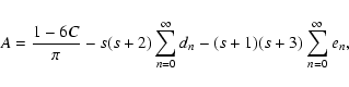 |
(43) |
where
![\begin{displaymath}%
\left\{
\begin{array}{l}
d_n = \frac{I_n}{4n^2-1},\\ [2mm]
e_n = \frac{J_n}{4n^2-1}\cdot
\end{array}\right.
\end{displaymath}](/articles/aa/full/2008/41/aa09682-08/img123.gif) |
(44) |
and C is the Catalan constant (half the area under the function ). Numerically, the constant in A is
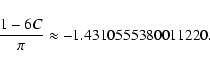 |
(45) |
Figure 2 shows the coefficient dn for s=-1.5 (in this case, dn=en). It follows that, for large n, dn and en behave like
 asymptotically, and so A approaches its converged value far more rapidly than by means of Eq. (34).
For
,
we then find:
![\begin{displaymath}
%
\begin{array}{l}
A_\Delta = \frac{1-6C}{\pi} + \gamma_{n_\...
... [2.5mm]
\qquad -(s+1)(s+3) \sum_{n=0}^\infty{e_n},
\end{array}\end{displaymath}](/articles/aa/full/2008/41/aa09682-08/img126.gif) |
(46) |
instead of Eq. (40), and for
,
this is:
![\begin{displaymath}%
\begin{array}{l}
A_1 = \frac{1-6C}{\pi} + \gamma_{n_1} \fra...
...]
{\scriptstyle n \ne n_1}\end{array}}^\infty{e_n},
\end{array}\end{displaymath}](/articles/aa/full/2008/41/aa09682-08/img127.gif) |
(47) |
instead of Eq. (42).
Depending on the exponent s of interest, a good approximation for A,
or A1 can be obtained by considering only the largest terms in the sum, i.e. all terms up to the rank
 or
or
 .
For astrophysical discs, s is around -1 meaning that we retain only the first term in Eq. (43). We then find the following approximation:
.
For astrophysical discs, s is around -1 meaning that we retain only the first term in Eq. (43). We then find the following approximation:
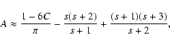 |
(48) |
whose accuracy is better than  for
for
 as Fig. 6 shows. For
 ,
we find from Eqs. (46) and (47):
,
we find from Eqs. (46) and (47):
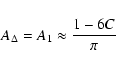 |
(49) |
which is in good agreement with the converged value given in Table B.
![\begin{figure}
\par\includegraphics[width=9cm,clip]{fig7hure09682.eps}\end{figure}](/articles/aa/full/2008/41/aa09682-08/Timg136.gif) |
Figure 7:
The exact potential for a power law disc with s=-1.5 ( thick line) compared to approximate values ( thin lines) found from Eq. (50) for N=0, 1, 2 and 3 (i.e. see Eqs. (52), (54), (55), etc.). The largest errors are found around edges. |
| Open with DEXTER |
7 Approximate formulae inside the disc
Equations (33), (39) and (41) contain three rapidly converging series that can be truncated to derive reliable approximations for the potential. For
 ,
only a few terms can be considered (see Sect. 6). Although many truncations are possible, we have noticed that the most accurate approximations of
for discs are obtained provided the coefficient A (or
or A1 depending on s) takes its converged value. Under these circumstances, the N-order approximation for the potential in region II becomes:
,
only a few terms can be considered (see Sect. 6). Although many truncations are possible, we have noticed that the most accurate approximations of
for discs are obtained provided the coefficient A (or
or A1 depending on s) takes its converged value. Under these circumstances, the N-order approximation for the potential in region II becomes:
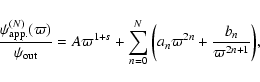 |
(50) |
which is, in its asymptotic limit:
 |
(51) |
As argued in Sect. 6.3, a reliable formula for the potential in astrophysical discs (for which
 )
is obtained by considering only the terms a0 and
)
is obtained by considering only the terms a0 and
 ,
in addition to the power law. At the lowest order, we thus have:
,
in addition to the power law. At the lowest order, we thus have:
 |
(52) |
where, in this case,
 (see Appendix B). Figure 7 compares this zero-order approximation with the exact potential for typical disc parameters. It follows that the relative deviation
 does not exceed 10%, the deviation being the largest close to the edges.
It is worth noting that the accuracy remains of the same order if coefficient A is determined by Eq. (48). This is convenient when the explicit dependence of
on s is required. Under this hypothesis, the potential becomes (see note 4):
| |
![$\displaystyle \psi(R) \approx - 2 \pi G \Sigma_{\rm out}a_{\rm out}\times \Bigg\{ \frac{1}{1+s} + \left[ 0.431 - \frac{1}{(1+s)(2+s)} \right]$](/articles/aa/full/2008/41/aa09682-08/img147.gif) |
|
| |
 |
(53) |
Figure 8 shows the accuracy of this formula in the
 -plane. We see that the relative deviation of 10% observed previously for s=-1.5 holds globally for s roughly in the range [-3,0]. This agrees with the fact that Eq. (48) produces values of A within a few percents for this range of exponents. The deviation can be reduced at the inner and outer edges provided additional terms are included (see below).
If necessary, more accurate expressions are obtained by accounting gradually for following terms (each acting as a smaller and smaller correction). For N=1, we have:
 |
(54) |
and for N=2, this is:
 |
(55) |
and so on. We note that Eq. (33) is particularly well suited to numerical computation since
can be determined by means of a recurrence procedure. A possible algorithm (not including the treatment of singular cases where
 )
is proposed in Appendix D.
)
is proposed in Appendix D.
![\begin{figure}
\par\includegraphics[width=9cm,clip]{fig8hure09682.eps}\end{figure}](/articles/aa/full/2008/41/aa09682-08/Timg152.gif) |
Figure 8:
Contour map showing the decimal logarithm of the relative error in the potential in the
-plane when
is approximated by Eq. (53). |
| Open with DEXTER |
8 Discs with no inner/outer edges
If the disc has no inner edge but a finite size (i.e.
and
), then the ODE is (see Huré & Hersant 2007):
 |
(56) |
It can be verified that the solution is still described by Eqs. (33) and (43), but the coefficients an and bn are:
![\begin{displaymath}%
a_n = \left \{
\begin{array}{l}
I_n, \quad {\rm in~region~II}\\ [2mm]
0, \quad {\rm in~region~III}
\end{array}\right.
\end{displaymath}](/articles/aa/full/2008/41/aa09682-08/img154.gif) |
(57) |
and
![\begin{displaymath}%
b_n = \left \{
\begin{array}{l}
0, \quad {\rm in~region~II}\\ [2mm]
-J_n, \quad {\rm in~region~III}.
\end{array}\right.
\end{displaymath}](/articles/aa/full/2008/41/aa09682-08/img155.gif) |
(58) |
If the disc is infinite but has an inner edge (i.e.
and
), then
 |
(59) |
where
 |
(60) |
is the new space variable,
 |
(61) |
and
 is a constant (this is not the potential at the inner edge). The analogue of Eq. (33) is:
 |
(62) |
where A is still given by Eq. (34),
![\begin{displaymath}%
a_n =\left \{
\begin{array}{l}
- I_n, \quad {\rm in~region~I}\\ [2mm]
0, \quad {\rm in~region~II}
\end{array}\right.
\end{displaymath}](/articles/aa/full/2008/41/aa09682-08/img161.gif) |
(63) |
and
![\begin{displaymath}%
b_n =\left \{
\begin{array}{l}
0, \quad {\rm in~region~I}\\ [2mm]
J_n, \quad {\rm in~region~II}.
\end{array}\right.
\end{displaymath}](/articles/aa/full/2008/41/aa09682-08/img162.gif) |
(64) |
If the disc is infinite, the ODE become homogeneous:
 |
(65) |
and the solution is a power law:
 |
(66) |
where R0 is some reference radius. In this case only, a self-similar surface density can rigorously be associated with a self-similar potential. The presence of edges destroys this property. We note that, for s=-1 (i.e. Mestel's disc), the derivation of the ODE requires a careful treatment. The integral form, i.e. Eq. (5), gives:
![\begin{displaymath}%
\psi(R) = - 4 G \Sigma_0 a_0 \left\{ 2C + \frac{\pi}{2} \le...
...{2n} + \ln \frac{a}{R} \right]_{a=a_{\rm out}}^{a=R} \right\}.
\end{displaymath}](/articles/aa/full/2008/41/aa09682-08/img165.gif) |
(67) |
We then have
 |
(68) |
This expression is compatible with Eq. (56a) when
(in this case, region III no longer exists and we have
 ).
).
In this paper, we have derived an exact expression for the gravitational potential in the plane of flat power-law discs as a solution of the ODE reported in Paper I. This expression is valid over the entire spatial domain and takes into account finite size effects. Inside the disc (the most difficult case to treat in general), it consists of three terms of comparable magnitude: a power law of the cylindrical radius R with index 1+s (where s is the exponent of the surface density) and two series of R and 1/R. In terms of convergence, our expression is by far superior to the multi-pole expansion method. Reliable approximations for the potential can be produced by performing fully controlled truncations. We have shown that the potential can be expressed by means of a simple function of R and s, which is valid to within a few percents in the range of exponents
 .
This formula should be sufficiently accurate for most astrophysical applications. If necessary, more accurate formulae can be developped by including successive terms. These results should help in investigating various phenomena where disc gravity plays a significant role.
.
This formula should be sufficiently accurate for most astrophysical applications. If necessary, more accurate formulae can be developped by including successive terms. These results should help in investigating various phenomena where disc gravity plays a significant role.
An interesting point concerns the case of discs for which the surface density is not a power-law function. As shown in Paper I, it is easy to reproduce numerically the potential when the profile  is a mixture of power laws. From an analytical point of view however, the construction of a reliable formula for
as compact as the one obtained here is not guaranteed at all. For instance, for an expansion of the form:
is a mixture of power laws. From an analytical point of view however, the construction of a reliable formula for
as compact as the one obtained here is not guaranteed at all. For instance, for an expansion of the form:
 |
(69) |
where s is an integer, each of the M+1 series
 should be truncated at a rank
 (see Eqs. (33) and (50)), which corresponds to an approximate formula for
containing about 2M(M+1) terms. The number of terms to consider can become prohibitively large when several power laws are required.
(see Eqs. (33) and (50)), which corresponds to an approximate formula for
containing about 2M(M+1) terms. The number of terms to consider can become prohibitively large when several power laws are required.
Acknowledgements
F. Hersant was supported by a CNRS fellowship which is gratefully acknowledged. We thank C. Baruteau. We thank the anonymous referee for valuable comments.
Appendix A: Vanishing coefficient A for s  {-3,0}
For
 ,
the coefficient is:
,
the coefficient is:
 |
(A.1) |
We notice that the first sum is the definite integral of u K(u), which is
To find the second sum, we compute the definite integral of K(u)/u2 in two ways. First, we have by direct integration (e.g. Gradshteyn & Ryzhik 1965):
Second, by replacing above
by its series representation, we also find:
Since
 ,
we have
,
we have
 |
(A.5) |
and so A=0 for s=-3 and s = 0.
Appendix B: Converged values of coefficient A, A1, and A for s [-4,1]
Table B.1:
Values of A (4th column) computed within the computer precision (double precision; about 16-digit) for different power law exponents s or s' (Cols 1 to 3) including those relevant for astrophysical applications (see also Fig. 5). Also given are the relative error on the coefficient (5th column) and the number of iterations (6th column) required.
Appendix C: Convergence acceleration for A
The coefficient A is given by a series whose convergence can be accelerated by considering an interesting property of the integral of
(e.g. Gradshteyn & Ryzhik 1965), namely:
 |
(C.1) |
where C is Catalan's constant. We can then write
where terms vary like 1/n3 for large n. A second convergence acceleration can be obtained by considering the complete elliptic integral of the second kind:
 |
(C.3) |
whose definite integral over the modulus x is:
 |
(C.4) |
We then have:
It follows that:
The second term in Eq. (34) gives:
But, from Eq. (C.4), we have:
and then:
| |
|
 |
|
| |
|
 |
(C.9) |
Finally, we have:
Appendix D: A basic algorithm
A possible algorithm is the following (see the text for cases where
 ):
):
- 1.
- disc parameters (see Sect. 2):
- set the inner edge

- set the outer edge

- set the outer surface density

- set the power law exponent s=???
 compute
  .
.
- 2.
- power-law coefficient A:
compute A (or
or A1 depending on s) at the computer accuracy (see Sect. 7); see Eqs. (43), (46) and (47), or use pre-computed converged values (see Appendix B).
- 3.
- radius
- set the radius R = ???
compute dimensionless variables  and X (depending on the region I, II or III).
- 4.
- initializations
- set  to 1; see Eqs. (13),
- set a0 to
 ;
see Eq. (31),
;
see Eq. (31),
- set b0 to
 ;
see Eq. (32),
;
see Eq. (32),
- set
to 0.
- 5.
- main loop on n
compute
from
 ,
,
compute an from an-1,
compute bn from bn-1,
compute
 and X2n+1,
update
to
 ;
see Eq. (50).
;
see Eq. (50).
- 6.
- power-law contribution
update
to
 ;
see Eq. (50).
;
see Eq. (50).
- 7.
- final potential value
change
for
 .
.
The loop ends after N steps; the accuracy of the potential value is then given by the next term (rank N+1).
-
Baruteau, C, & Masset, F. 2008, ArXiv e-prints, 801
(In the text)
- Bisnovatyi-Kogan,
G. S. 1975, SVR Let., 1, 177
- Clement,
M. J. 1974, ApJ, 194, 709 [NASA ADS] [CrossRef]
- Collin-Souffrin, S., &
Dumont, A. M. 1990, A&A, 229, 292 [NASA ADS]
- Dubrulle, B.
1992, A&A, 266, 592 [NASA ADS]
- Durand, E. 1953,
Electrostatique, Vol. I, Les distributions (Ed. Masson)
(In the text)
- Edgar, R. G.
2007, ApJ, 663, 1325 [NASA ADS] [CrossRef]
- Evans, N. W.
1994, MNRAS, 267, 333 [NASA ADS]
- Evans,
N. W., & Read, J. C. A. 1998, MNRAS, 300,
83 [NASA ADS] [CrossRef]
- Gradshteyn,
I. S., & Ryzhik, I. M. 1965, Table of integrals,
series and products (New York: Academic Press), 4th edn., ed. Yu. V
Geronimus, & M. Yu. Tseytlin
(In the text)
- Hayashi, C. 1981,
Prog. Theor. Phys. Suppl., 70, 35 [NASA ADS] [CrossRef]
(In the text)
- Hughes, A. M.,
Wilner, D. J., Qi, C., & Hogerheijde, M. R. 2008,
ArXiv e-prints, 801
(In the text)
- Hunter, Jr.,
J. H., Ball, R., & Gottesman, S. T. 1984, MNRAS, 208,
1 [NASA ADS]
- Huré, J.-M. 1998,
A&A, 337, 625 [NASA ADS]
- Huré, J.-M., &
Hersant, F. 2007, A&A, 467, 907 [NASA ADS] [CrossRef] [EDP Sciences]
(In the text)
- Huré, J.-M.,
Richard, D., & Zahn, J.-P. 2001, A&A, 367, 1087 [NASA ADS] [CrossRef] [EDP Sciences]
(In the text)
- Kellogg,
O. D. 1929, Foundations of Potential Theory (New-York:
Frederick Ungar Publishing Company)
(In the text)
- Mestel, L. 1963,
MNRAS, 126, 553 [NASA ADS]
(In the text)
- Piétu, V.,
Dutrey, A., & Guilloteau, S. 2007, A&A, 467, 163 [NASA ADS] [CrossRef] [EDP Sciences]
(In the text)
- Pringle,
J. E. 1981, ARA&A, 19, 137 [NASA ADS] [CrossRef]
- Richard,
D., & Zahn, J.-P. 1999, A&A, 347, 734 [NASA ADS]
- Rybicki,
G. B., & Lightman, A. P. 1979, Radiative processes in
astrophysics (New York: Wiley-Interscience), 393 [NASA ADS]
(In the text)
- Semerák, O.
2004, Class. Quant. Gravity, 21, 2203 [NASA ADS] [CrossRef]
- Shakura, N. I., &
Sunyaev, R. A. 1973, A&A, 24, 337 [NASA ADS]
- Stone,
J. M., & Norman, M. L. 1992, ApJS, 80, 753 [NASA ADS] [CrossRef]
- Zhao, H., Carollo,
C. M., & de Zeeuw, P. T. 1999, MNRAS, 304, 457 [NASA ADS] [CrossRef]
Copyright ESO 2008
![\begin{figure}
\par\includegraphics[width=9cm,clip]{fig2hure09682.eps}\end{figure}](/articles/aa/full/2008/41/aa09682-08/img65.gif)
![\begin{figure}
\par\includegraphics[width=9cm,clip]{fig3hure09682.eps}
\end{figure}](/articles/aa/full/2008/41/aa09682-08/img92.gif)
![\begin{figure}
\par\includegraphics[width=9cm,clip]{fig5hure09682.eps}
\end{figure}](/articles/aa/full/2008/41/aa09682-08/img103.gif)
![\begin{figure}
\par\includegraphics[width=8.5cm,clip]{fig6hure09682.eps}\end{figure}](/articles/aa/full/2008/41/aa09682-08/img128.gif)
![\begin{figure}
\par\includegraphics[width=9cm,clip]{fig7hure09682.eps}\end{figure}](/articles/aa/full/2008/41/aa09682-08/img136.gif)
![\begin{figure}
\par\includegraphics[width=9cm,clip]{fig8hure09682.eps}\end{figure}](/articles/aa/full/2008/41/aa09682-08/img152.gif)


![$\displaystyle \frac{2}{\pi} \left[ - \frac{{\vec E}(u)}{u}\right]_0^1,$](/articles/aa/full/2008/41/aa09682-08/img183.gif)
![$\displaystyle - \frac{2}{\pi} \left[ {\vec E}(1) - \lim_{u \rightarrow 0} \frac{{\vec E}(u)}{u} \right],$](/articles/aa/full/2008/41/aa09682-08/img184.gif)
![$\displaystyle - \gamma_0 \left[1 - \lim_{u \rightarrow 0} \frac{1}{u} \right] + \sum_1^\infty{\frac{\gamma_n}{2n-1}},$](/articles/aa/full/2008/41/aa09682-08/img189.gif)

![$\displaystyle \qquad \qquad\left. \quad+\frac{1}{(2n+1)(2n-1)}\right] - \sum_{n=0}^\infty{\frac{\gamma_n}{(2n+1)(2n-1)}}$](/articles/aa/full/2008/41/aa09682-08/img201.gif)


![$\displaystyle \left.\qquad \qquad-\frac{1}{(2n+1)(2n-1)}\right] + \sum_{n=0}^\infty\frac{\gamma_n}{(2n+1)(2n-1)}$](/articles/aa/full/2008/41/aa09682-08/img210.gif)