A&A 489, 755-762 (2008)
DOI: 10.1051/0004-6361:20079052

Stability and mode analysis of solar coronal loops using thermodynamic irreversible energy principles

II. Modes in twisted non-isothermal magnetic field configurations

A. Costa^1,2 - R. González^2,3,4

1 - Instituto de Astronomía Teórica y Experimental (IATE-CONICET), Córdoba, Argentina
2 - Instituto de Astronomía y Física del Espacio (IAFE-CONICET) Buenos Aires, Argentina
3 - Universidad Nacional de General Sarmiento (UNGS), Argentina
4 - Departamento de Física (FCEyN-UBA) Buenos Aires, Argentina

Received 12 November 2007 / Accepted 26 June 2008

Abstract
Aims. We study the stability and modes of non - isothermal coronal loop models with different intensity values of equilibrium twisted magnetic field.
Methods. We use an energy principle obtained by means of non - equilibrium thermodynamic arguments. The principle is expressed in terms of Hermitian operators and enables us to consider the coupled system of equations, the balance of energy equation and the equation of motion, to obtain modes and eigenmodes in a spectrum ranging from short to long-wavelength disturbances without using weak varying approximations of the equilibrium parameters. Long-wavelength perturbations introduce additional difficulties because the inhomogeneous nature of the medium produce disturbances corresponding to continuous intervals of eigenfrequencies, which cannot be considered as purely sinusoidal.
Results. We analyze the modification of periods, modes structure, and stability when the helicity, the magnetic field strength, and the radius of the fluxtube are varied. The efficiency of the damping due to the resonant absorption mechanism is analyzed in terms of modes that can either impulsively release or store magnetic energy.
Conclusions. We find that the onset of the instability is associated with a critical value of the helicity and the magnetic energy content has a determinant role on the instability of the system with respect to the stabilizing effect of the resonant absorption mechanism.

Key words: Sun: corona - Sun: oscillations - Sun: magnetic fields

1 Introduction

1.1 Variational principle

A crucial requirement of any theoretical model of coronal structures is to describe the stability and evolution of far-from-equilibrium states that are responsible for the characteristic rich topology and dynamics of the solar corona. This requires the coupling of thermal and mechanical equations. Different stability analyses of solar structures can be found in the literature, generally restricted to special types of perturbations and specific equilibrium models. These include, models that consider adiabatic configurations such as those analyzed by means of the classical criterion of Bernstein (1958), or those that assume static equilibrium and analyze the thermal stability. In the application of Bernstein's criterion, the adiabatic assumption implies that the energy balance equation is not required and dissipation is therefore impossible. The assumption of static models is also a strong, and often unjustified, restriction for open systems.

We apply an energy principle to analyze the stability of solar coronal loops when helical modes are present. The principle was developed in previous papers (Paper I: Costa & González 2006; Costa et al. 2004; see also Sicardi Schifino et al. 1991) using a general procedure of irreversible thermodynamics - based on firmly established thermodynamic laws - that can be understood as an extension of Bernstein's MHD principle to situations far from thermodynamic equilibrium.

In Paper I and Costa et al. (2004), we showed how to obtain the variational principle for solar coronal structures from the equations that describe the dynamics of the system. The method consists of obtaining a Lyapunov function, also known as a generalized potential, that represents the mathematical expression of the stability conditions. The principle is subject to physically reasonable requirements of hermiticity and antihermiticity over the matrices. For a more detailed presentation, see Paper I and references therein.

1.2 Solar coronal loops

MHD loop oscillations in the corona are known to be strongly damped, with decaying times of a few periods $N_{\rm p}\approx 2{-}7 \$ periods. While thermal conduction, and radiative cooling mechanisms, could be the responsible for the damping of pure MHD slow magnetoacoustic mode oscillations, they are unimportant in shaping the MHD fast modes. Resonant absorption and phase mixing appear more promising in means of accounting for the rapid decay (Halberstadt & Goedbloed 1994, hereafter HG; Goossens et al. 2002) of the ideal fast oscillations of these strongly inhomogeneous and structured plasma systems. Inhomogeneous equilibrium distributions of plasma density and temperature varying continuously across the magnetic field produce plasma waves with continuous intervals of eigenfrequencies. The presence of the Alfvén ideal MHD continuum in a thin edge layer is inferred from the highly anisotropic character of the fast magnetoacoustic waves that generates a peak in the amplitudes where the perturbation develops large gradients and the absorption has maxims. However, there is another type of continuum commonly known as slow magnetosonic continuum associated with the inhomogeneity of the equilibrium parameters along the axis of the loop (see Paper I). These inhomogeneities are associated, for example, with changes in the density concentration at the loop basis. If the magnetic field is twisted, the inhomogeneities lead to the coupling of Alfvén and slow magnetosonic continuum modes (Belien et al. 1997).

The resonant absorption mechanism of wave heating consists of the non-dissipative transfer of wave energy from the collective line-tied wave with fast discrete eigenvalues (kinetic energy of the fast radial component) to a local resonant mode in the Alfvén continuum, (kinetic energy of the azimuthal component), which is then dissipated in an enhanced manner. Then, the continuum oscillations are converted into heat by dissipative processes; since the medium has large gradients in the Alfvén speed, the oscillations of neighboring field lines become out-of-phase and shear Alfvén waves lead to enhanced viscous and ohmic dissipation (see Heyvaerts & Priest 1983, for the linear regime, and Nakariakov et al. 1997, for the nonlinear one). The mode conversion from the collective to the local mode occurs in a time that is non-dissipative and generally far shorter than the second timescale that is related to the dissipative damping of the small-scale perturbations of the local mode in the resonance layer (Roberts 2000; Van Doorsselaere et al. 2004).

The entire temporal pattern description of modes that exhibit a combination of global (discrete line-tied fast eigenmode) and localize (Alfvén continuum mode) behavior is known as quasi-mode. The mixed nature of the modes is not only due to the temporal behavior but also to the boundary value problem, which produce a spatial behavior that is of a mixed nature, i.e. coronal loops with line-tying constraints that cannot support pure waves, i.e. Alfvén, slow or fast magnetoacoustic modes. HG studied the mixed spectral description of coronal loops (i.e. the resulting superposition of basic waves that adjust the line-tied condition) without assuming a straight magnetic field and forcing the loop to follow the photospheric velocity perturbations. They found that pure Alfvén and pure slow modes are obtained as singular limiting cases of the spectra of Alfvén-fast or slow-fast modes, where the fast components are localized in a photospheric boundary associated with the line-tied condition. The coronal part of the loop which acts as a resonant cavity of both large Alfvén and fast components of small but rapidly varying amplitudes located in the photospheric boundary layer. They found that the heating of coronal loops by resonant absorption is due to the line-tied Alfvén continuum that no longer depends on the poloidal magnetic field; the corresponding eigenmodes also have a global ballooning feature, which is characterized by an accumulation point given by the Alfvén frequency. In Goedbloed & Halberstadt (1993, hereafter GH), a variational principle, based on Bernstein's principle, was obtained to derive the Alfvén and slow continuum frequencies in a line-tied inhomogeneous cylinder. Stability considerations led the authors to the global stability of coronal loops.

Following results of Paper I, we apply our energy principle to consider the stability and mode structure of loop inhomogeneous coronal models of non-vanishing helicity. Our principle has the advantage that it does not require a WKB approximation and that, as afore mentioned, it allows the consideration of the coupling of the thermal and mechanical equations that are necessary to analyze far from equilibrium states.

2 The MHD stability criterion for coronal structures

Solar coronal conditions with large Reynolds numbers are well described by ideal MHD plasma models (i.e. infinite electrical conductivity $\sigma \gg 1$ of vanishing viscosity and ohmic dissipation). The fundamental equations that we consider are therefore the mass conservation equation, the perfect gas law or state equation for a fully ionized H plasma, and the induction equation with vanishing magnetic diffusivity due to the conductivity properties. The energy balance equation takes the form:

$$\frac{\rho^{\gamma}}{(\gamma-1)}\frac{\rm D}{\rm D t}\Big(\frac{p}{\rho^{\gamma}}\Big)=-\nabla\cdot\vec{F}_{\rm c}-L_{\rm r}+H$$ (1)

$\vec{F}_{\rm c}$ is the heat flux due to particle conduction along the loop, $L_{\rm r}$ is the net radiation flux, and H the heating function, which was chosen as in Paper I: $H = h \rho + H_{0}$. Equation  (1) expresses the fact that the gain in particle energy (internal plus kinetic) is due to the external heating sources represented by the heating function, heat flow, and radiation losses; all other heating sources were considered as vanishing terms implying that the optically thin assumption holds. We note that the non-ideal contribution in the energy equation (L) is associated with the open character of the loop system.

When a linearization about a nonlinear equilibrium or stationary state is performed and a procedure has been completed in which the hermiticity requirements are fulfilled, the generalized energy principle and the respective frequencies are obtained (Paper I and Costa et al. 2004) as:

$$\delta^{2} W_{\rm p} =\frac{1}{ 2}\int ( \vec{\xi}^{*} \beta ... ... +T_{1}^{*}B\vec{\xi} -\vec{\xi}^{*}BT_{1}){\rm d}^{3}x\geq 0.$$ (2)

$$\omega^{2} =- \frac{\int ( \vec{\xi}^{*} \beta F\vec{\xi} + T... ...}x}{\int (\vec{\xi^{*}} \beta \rho_{0}\vec{\xi} ){\rm d}^{3}x}$$ (3)

with the same normalization condition as in Paper I. F is the known Bernstein operator for the system, $\xi$ and T₁ are the motion and temperature perturbations and operators A and B are as in Paper I. For the non-dissipative cases (L=0 or equivalently T₁=0), the final expressions (discarding the presence of factor $\beta$ that appears in the equations to fit the Hermitian and anti-Hermitian conditions) are reduced to the well-known Bernstein MHD energy principle and its respective frequencies.

3 Application to an inhomogeneous loop model of non-vanishing helicity

On the one hand, the azimuthal component of the loop perturbation is believed to be one of the principle responsible of resonant absorption and damping of ideal oscillations. On the other hand, this component is associated with the storage of magnetic energy in systems of non-vanishing helicity that is eventually released by instabilities. Therefore, we are interested in analyzing changes in the stability of non-homogeneous loops affected by helical perturbations; loops have inhomogeneous distributions of plasma density and temperatures, affected by body modes and non-vanishing helicity. The Alfvén, slow, and fast magnetoacoustic cylinder modes can then no longer be associated with the azimuthal, longitudinal, and radial components, respectively. The observational importance of helical modes cannot be neglected and it is not understood well how helicity affects important physical features of mode oscillations (e.g. damping mechanisms, stability and periods). However, a mode classification can be accomplished by the analysis of mode variations, described in an orthogonal basis, while helicity is varied. The basis is formed by orthogonal displacements both parallel and perpendicular to the magnetic field, and radial displacement (and perpendicular to the surface of the tube) that is of observational interest.

The fundamental modes are observationally and energetically more important in general than their harmonics. In these global modes, the inhomogeneous nature of the medium cannot be ignored: it determines the structure of the disturbance, which we cannot assume to be sinusoidal; this implies that the traditional normal mode analysis cannot be applied in this case, i.e. at least a WKB approximation, with parameters that vary weakly compared with the scale of typical wavelength, is required. The occurrence of either an infinitely degenerate eigenvalue or an accumulation point that produces a continuous spectrum are associated with inhomogeneities. We consider two types of inhomogeneities: the inhomogeneity of the equilibrium parameters along the loop axis, and the inhomogeneity across the loop axis when the radius is varied. As a first order approximation, we neglect the effect of gravitational stratification and confine the analysis to characteristic spatial scales lower than the pressure scale height in the solar corona. To analyze the stability and to obtain the frequencies and modes, the physical quantities in Eqs. (2) and (4) must be calculated along the loop structure.

3.1 Mechanical equilibrium

To determine an equilibrium configuration, we assume force-free equations. This assumption is justified for coronal conditions due to the fact that in plasmas of low $\mathcal{\beta}$ (gas pressure over the magnetic pressure), the pressure gradient can be neglected in comparison with the Lorentz force. For the chromosphere and photosphere, the force-free approximation may not be a good one. However, it is a widespread supposition (Ruderman 2007): perturbed systems are believed to relax to new force-free, minimum energy states and chromospheric conditions appear to be well described by force-free models from an altitude of $4. \times \ 10^{5}$ m (Aschwanden 2004, Chap. 5).

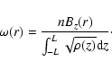
Coronal loops are modeled as thin cylindrical fluxtubes, where the curvature and related forces are neglected so that the cylindrical geometry can be applied. The fluxtube is assumed as line-tied to the photospheric plasma through its footpoints, which are forced to follow the photospheric velocity perturbations. The random velocity field creates a vorticity that in general twists the coronal fluxtubes. A relation between the helical twist and the force-free parameter can therefore be derived as follows (e.g. Sturrock 2004). The coronal loop model is obtained from the equations

$$\nabla \times \vec{B}_{0}=\alpha(r) \vec{B}_{0} \ \ \ \vec{j} \times \vec{B}_{0}=0.$$ (4)

Since $\vec{B}_{0}$ is force-free, $\nabla p=0$ everywhere and has a constant value along the loop. We consider a straight cylinder of a nonuniform distribution of density and temperature and a uniform twist over an initially non-rotated field $\vec{B}=(0,0,B_{z}),$ which produces the unperturbed magnetic field

$$\vec{B}_{0} = (B_{r}, B_{\phi} , B_{z})=(0,B_{0} b r /\Delta,B_{0} /\Delta)$$

with $\Delta=1+b^{2}r^{2}$ and $b=2 \Pi N_{\rm t}/L$ (where $N_{\rm t}$ is the number of turns over the cylinder length L). Then,

$$\frac{B_{\phi}}{B_{z}}=\frac{r \partial \phi}{\partial z}=\f... ...r 2 \pi N_{\rm t}}{L}=br \\ \alpha(r) =\frac{2b}{\Delta}\cdot$$ (5)

We assume a given value of the cylinder radius r=R, and the line element is therefore a function of the coordinate z such that s=s(z). The dependence of the coordinates with the radial component is taken into account by considering different values of the radius R

$${\rm d}s^{2}=R^{2}{\rm d} \phi^{2}+{\rm d}z^{2}=\left( 1+R^{2} b^{2}\right) {\rm d}z^{2} =\Delta {\rm d}z^{2}.$$ (6)

3.2 Thermal equilibrium

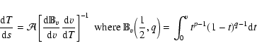
The thermal equilibrium is obtained, as in Paper I, by assuming that L=0 in the balance energy Eq. (1). The procedure developed consists of obtaining the function of the temperature along the arc element s by integrating Eq. (1) with the constraint L=0 and the boundary conditions of temperature at the bottom $T_{\rm b}=10^{4}$ K and temperature at the top $T_{\rm t}=10^{6}$ K. The following expression (see Chap. 6 of Priest 1982) is obtained

$$\left[\frac{{\rm d}T}{{\rm d}s}\right]^{2}=\frac{p^{2}\chi}{2... ...}{2}} \left[1 - \Big ( \frac{T}{T_{t}}\Big)^{2-\alpha}\right],$$ (7)

which has to be inverted to obtain T=f^-1(s) (Arfken & Weber 1995) as

$$\frac{{\rm d}T}{{\rm d}s}=\mathcal{A}\left[\frac{{\rm d}\math... ...\Big(\frac{1}{2},q\Big)=\int_{0}^{v}t^{p-1}(1-t)^{q-1}{\rm d}t$$ (8)

$${\rm with} ~~p= \ \frac{1}{2}; \ v=1-(T/T_{\rm t})^{2-\alpha}; \ q=\left(\frac{\alpha}{2}+\frac{3}{4}\right) \ (2-\alpha)+1$$

$$\mathcal{A}=(2-\alpha)T_{\rm t}^{\frac{\alpha}{2}-\frac{11}{4... ...\alpha+\frac{3}{2}\Big)k_{\rm B}^{2}\Big)\Big)^{\frac{1}{2}}.$$

We use $\alpha=-\frac{1}{2}$ so $q=\frac{6}{5}$ to calculate the modes numerically,

$$s=\frac{1}{\mathcal{A}} \mathbb{B}_{v}\Big(\frac{1}{2}, \frac... ... ( \frac{p^{2}\chi}{2k_{0}k_{\rm B}^{2}}\Bigg)^{ \frac{1}{2}}.$$

From the boundary conditions, $\upsilon =0;$ the constant value of the heating function therefore becomes $H_{0}= 7 p^{2} \chi T^{\alpha -2}_{\rm t}/\left(8 k_{\rm B}^{2}(\alpha +\frac{3}{2})\right).$

3.3 The perturbation

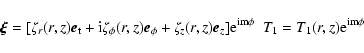
To calculate the stability and structure of the modes, the general perturbation along the equilibrium magnetic field is written to be

$$\vec{\xi}=[\zeta_{r}(r,z) \vec{e}_{\rm t}+{\rm i} \zeta_{\phi... ... e}^{{\rm im}\phi} \ \ T_{1}=T_{1}(r,z) {\rm e}^{{\rm im}\phi}$$ (9)

with r=R. The $\phi$ dependence only appears in the exponents that multiply the perturbation; the integration with respect to this coordinate is straightforward. By representing the equilibrium functions of the different quantities with a 0 sub-index, and defining

$$\vec{e}_{\rm t}=(Rb \vec{e}_{\phi}+ \vec{e}_{z} )/ \sqrt{\Del... ...cdot\nabla) \rho_{\rm t}=\frac{m_{\rm p}}{k_{\rm B}T_{\rm t}}$$

where $\vec{e}_{\phi}, \vec{e}_{z}$ are cylindrical versors and $\vec{e}_{\rm t}$ the tangential versor, we obtain a non-dimensional expression for the energy principle of Eq. (2)

$$\delta^{2} W_{\rm p}= \delta^{2} W_{\rm c}+\delta^{2} W_{\rm m}+\delta^{2} W_{\rm hc}+\delta^{2} W_{\rm r}$$ (10)

where $\delta^{2} W_{\rm c}$ is the generalized potential energy associated with the compressional terms, $\delta^{2} W_{\rm m}$ corresponds to the magnetic contributions, $\delta^{2} W_{\rm hc}$ corresponds to the heat conduction terms, and $\delta^{2} W_{\rm r}$ to the radiative contributions. The explicit form of these functions are given in the Appendix. The Bernstein generalized potential energy corresponds to the magnetic contribution and part of the compressional one. In the generalized version of the energy principle, additional terms appear in the $\delta^{2} W_{\rm c}$ term, and $\delta^{2} W_{\rm hc}$ and $\delta^{2} W_{\rm r}$ are entirely new terms.

4 Results and discussion

Convective motion of the photosphere is believed to provide energy that is stored in twisted magnetic coronal fields, producing long-lived coronal structures, until it is released by instabilities (Raadu et al. 1988; Vrsnak et al. 1991). On the other hand, continuous spectra are often associated with stability. Unstable modes are often assumed to have a discrete spectrum (see Freidberg 1982; or Priest 1982). There are two types of possible continuous spectra in this problem. The inhomogeneity of the equilibrium parameters along the loop axis produces a continuum that couples whith the Alfvén continuum (Belien et al. 1997); when the disturbances considered are comparable to the inhomogeneous characteristic wavelength, stable eigenvalues can give rise to a continuous spectrum (L/2, the equilibrium structure in the z component). This is the case studied in Paper I. On the other hand, GH established, for non vanishing helicity systems, that there is a continuous spectrum associated with the line-tied Alfvén resonance that produces damping and heating by the resonant absorption mechanism and directly relates to the stability of loops. They also described how the resonant singular limit $\omega$, could be obtained from the class of physically permissible solutions,

$$\omega(r)=\frac{nB_{z}(r)}{\int_{-L}^{L}\sqrt{\rho(z)}{\rm d}z}\cdot$$ (11)

This resonance occurs because of the absence of an explicit dependence on the azimuthal magnetic field component ( $B_{\varphi}$).

To understand the conditions in which the mechanism can dominate and describe the different scenarios such as the driving of the instability or the damping of mode oscillations, it is critical to gain knowledge about the dynamics and energetic contribution of twisted structures. The implications of the twisting in theoretical and observational descriptions are poorly known; for example, the modification of the dispersion relation is unclear and observational data are inferred indirectly.

We have focused our attention on describing the changes in periods, stability, and mode structure of coronal loops when the helicity, the magnetic field intensity, and the radius are varied. For loops of vanishing helicity, it is well established that the Alfvén line-tied resonance continuum is responsible for the damping of kink (m=1) quasi-modes via the transfer of energy from the radial component into the azimuthal one, i.e. from discrete global modes into the local continuum modes where phase mixing can take place. The twisting of the magnetic field leads however to the coupling of MHD cylindrical modes that make it difficult to provide a classification in terms of the behavior of pure-like modes.

To calculate modes and frequencies, we followed the schematic procedure described in Paper I and in Galindo Trejo (1987). We used a symbolic manipulation program to integrate the equations and the perturbations in $\delta^{2}W_{\rm p}$ were expanded in a six dimensional-Fourier basis in terms of the independent coordinate z that adjusts to boundary conditions, i.e. the four perturbed components (Eq. (9)) were expanded in a six mode basis to obtain 24 eigenvalues and eigenvectors for each of the helicity and the magnetic field values. Only the first eighteen eigenvalues were considered (the others are more than two orders of magnitude smaller and accumulate at zero; the eigenvectors are also vanishingly small). A quadratic form for $\delta^{2}W_{\rm p}$was therefore obtained and minimized with the Ritz variational procedure. A matrix discrete eigenvalue problem, affected by a normalization constraint, was obtained. From the resulting modes and the generalized potential energy (Eq. (2)): $\delta^{2}W_{\rm p}\geq0$ the stability of each mode was determined.

The coronal loop parameters used were L=10¹⁰ cm (or 100 Mm), $T_{\rm b}=10^{4}$ K $T_{\rm t}=10^{6}$ K, $n_{\rm e}=10^{8}$ cm^-3, $p_{\rm t} =2k_{\rm B}T_{\rm t}$ and $\rho_{\rm t}=m_{\rm p}p_{\rm t}/k_{\rm B}T_{\rm t}$. Frequencies and modes were calculated for two different values of the magnetic field B₀=10 G and 100 G, and for three different values of the helicity $b=3.1 \times 10^{-8}, 3.1\times 10^{-7}, 1.9 \times 10^{-6}$ which correspond to the adimentional values $b_{\rm a}=2.8, \ 28, \ 170$ with $N_{\rm t}=0.45, \ 4.3, \ 13.7$, and $N_{\rm t}$ is the number of turns over the cylinder length. These helicity values, defined as weak, moderated, and strong helicity, respectively correspond to the classification given in Aschwanden (2004, Chap. 5). The adimensional radius was initially chosen to be R=0.01. We summarize below the conclusions obtained from the data analysis displayed in three tables.

Table 1: Eighteen first periods associated with stable (S) and unstable (U) eigenvalues (minutes) for A) left panel: B₀=10 G with A1) left column: weak helicity, A2) middle column: moderate helicity, A3) right column: strong helicity and B) right panel: B₀=100 G with B1, B2, B3 the same as in A. Higher order modes were not considered.

Table 1 shows the periods (in minutes) for weak, moderate, and strong helicity for two values of the magnetic field intensity B₀=10 G and 100 G (left and right panel, respectively). S and U letters indicate the stable-unstable character of the modes. From the table, we see that:

I)

Weak helicity modes are stable. This is in accordance with the analytic results by Ruderman (2007), who studied nonaxisymmetric oscillations of a thin twisted magnetic tube with fixed ends in a zero-beta plasma.

II)

Higher modes have an accumulation point at zero, indicating the presence of a continuum spectra of stable modes (as in Paper I). We note that, calculus performed on a discrete basis, as in our case, provide spectra that are necessarily discrete. An accumulation of discrete eigenvalues therefore suggests a stable continuum spectrum.

III)

The B₀=10 G case has larger periods than the B₀=100 G one. For moderate and strong helicity, the eigenvalues of the first panel follow a scaling law with that of the second one i.e. they scale with the magnetic field intensity exactly as the Alfvén speed does $P_{10~{\rm G}}\simeq 10 P_{100~{\rm G}}$.

IV)

As HG and GH found, we note a clustering in the spectra associated with the change from real to imaginary eigenvalues (and viceversa). There is a pronounced change (in the spacing of the periods or/and in the stability) between the sixth mode and the seventh mode. This is noted by a double line in Table 1 and related to the importance of the parallel component with respect to the perpendicular component (see Table 2). Up to period number ten, real - imaginary eigenvalues in the first panel (B₀=10 G) correspond to real-imaginary ones in the second panel (B₀=100 G). Apart from high order periods n>10, the imaginary stable eigenvalues became imaginary unstable ones when the helicity is increased from weak to moderate. For B₀=10 G and weak and moderate helicity cases, there are five different groups of periods ( P₁-P₆;P₇-P₁₀;P₁₁-P₁₂;P₁₃-P₁₄;P₁₅- P₁₈) (see also Table 2). The clustering is more difficult to establish i.e. the differences are less pronounced with increasing magnetic field intensity and higher order periods.

To compare our results with those given by previous authors, we calculated the frequency of Eq. (11) for our modes. We found that all periods, apart from P₁-P₆ weak helicity modes, satisfy the relation and therefore belong to the Alfvén continuum spectrum justifying the scaling law described in III. As found by HG, we conclude that the change in the real-complex character of the P₆-P₇ eigenvalues is associated with the existence of an accumulation point of the resonant Alfvén continuum, however we find that this change is not necessarily related to a change in the stability as they claimed. We note that all modes with weak helicity are stable (even the imaginary ones); in all other cases, the imaginary character of the eigenvalues is associated with instability. The continuum stable eigenvalue conjecture is however still valid (Freidberg 1982; Priest 1982); it applies to a spectrum with an accumulation point at zero; we found stable modes for all the helicity values and for the two magnetic field values with P_n>14. We note that the analysis of the remaining stable modes is of interest because, depending on the relative characteristic times of stable and unstable modes, the stable ones could be active and accessible to observations.

The presence of at least one unstable mode implies that the equilibrium state is unstable. Taking into account the entire range of stable modes, we are able to confirm previous results; we therefore conclude that field configurations with some degree of twisting provide a stabilizing effect, allowing the storage of magnetic energy (Raadu 1972). This implies that when the helicity is augmented the stable weak case becomes unstable, which suggests that a critical value exists.

In Paper I, we derived only one unstable mode. This was classified as a slow magnetoacoustic mode bacause of the almost longitudinal character (parallel to the magnetic field) of the wavevector perturbation and the fact that the period did not vary with magnetic field intensity resembling acoustic waves of sound speeds, $v_{\rm s}$, independently of the magnetic field. The characteristic unstable time obtained in Paper I was $\tau_{\rm u}=36$ min, which corresponded to a typical slow magnetoacoustic fundamental period with a characteristic wavelength of the order of the loop length L/2. We also obtained a continuous set of stable modes; these were classified as fast magnetoacoustic modes because of the significance of the component orthogonal to the magnetic field and the fact that the eigenvalues scaled with the intensity of the magnetic field as $P_{11~{\rm G}}\simeq 10 P_{100~{\rm G}},$ which resembles the dependence of the Alfvén waves $v_{\rm A} \sim B_{0}.$

Table 2 (first panel) displays the resulting features associated with the relative intensity of the components both parallel and perpendicular to the field (where $(\xi_{\parallel},\xi_{\perp},\xi_{r})$ is an orthogonal basis) and their classification as either slow-like (S) or fast-like (F). The relative phase between the components is also indicated in the table by P (in phase) and IP (inverted phase). Table 2 (second panel) also shows the intensity relationship between the cylindrical components. To classify the modes and then compare them with the slow and fast magnetoacoustic modes obtained in Paper I, we calculated the cylindrical mode components and also both the components tangential and normal to the field ( $\xi_{\parallel}=(Rb\xi_{\phi}+\xi_{z})/\Delta; \xi_{\perp}= (\xi_{\phi}-Rb\xi_{z})/\Delta$). We are interested in the $\xi_{\parallel}$, $\xi_{z}$, $\xi_{r}$, $\xi_{\perp},$ and $\xi_{\phi}$ components because: when the helicity is weak, the $\xi_{\parallel}$ component is expected to play the slow-mode role of $\xi_{z}$in Paper I; and the $\xi_{r}$ component is related to the fast modes and determines the resonant absorption mechanism when uniform cylindrical flux tubes are considered by the transfer of energy to the $\xi_{\phi}$ component. When helicity and inhomogeneous distribution of equilibrium parameters are present, it is worth investigating the transfer of energy from the $\xi_{r}$ component to the others. In this case, the resonant damping of global oscillations occurs by converting the kinetic energy of the radial component into kinetic energy of the $\xi_{\parallel}$ and $\xi_{\perp}$ components; both components then form the plane orthogonal to $\xi_{r}$, which is equivalent to the plane formed by $\xi_{\phi}$ and $\xi_{z}$.

Table 2: First panel: intensity relationship between the tangential and normal field components of the eighteen first periods for B₀=10 G, for weak (first column), moderate (second column), and strong helicity (third column) cases. The (P) indicates in phase and (IP) indicates inverted phase. Second panel: intensity relationship between the cylindrical components of the eighteen first periods for B₀=10 G, for weak (first column), moderate (second column) and strong helicity (third column), cases.

By analyzing the component amplitudes of the P₁-P₆ modes with respect to the P₇-P₁₈ modes in the weak helicity case (the real and imaginary eigenvectors of Table 1, respectively), we are able to classify the first modes as slow-like modes because: I) their tangential components $\xi_{\parallel}$are at least an order of magnitude larger than the normal ones $\xi_{\perp}$; II) as the helicity is weak $\xi_{\parallel}\approx \xi_{z}$ and $\xi_{r}\rightarrow 0; \xi_{\phi}\rightarrow 0$, the wavevector is almost tangential to the magnetic field; III) they have a larger characteristic time and a shorter characteristic speed than the imaginary eigenvectors. In contrast, imaginary eigenvalues are associated with large values of the $\xi_{r}$ component and $\xi_{\perp}$ component (due to large values of $\xi_{\phi}$: see the second panel, Table 2) , and small values of the $\xi_{\parallel}$ and $\xi_{z}$ components. As in Paper I, when the eigenvalues change form real to imaginary, the period declines significantly and the type of mode varies from slow to fast magnetoacoustic. In Paper I, we found that the acoustic mode has the same eigenvalue for both magnetic field intensities; here, in contrast, the modes are affected by the strengthening of the magnetic field that produces an-order-of-magnitude shorter period than in the non-helicity case. The $\xi_{\parallel}$ and $\xi_{\perp}$ components are in an inverted phase for real eigenvector modes and in phase for imaginary eigenvector modes.

For moderate helicity, the overall description is similar but all cases have non vanishing $\xi_{\phi}$ components and all periods have a resonant line-tied continuum. As mentioned, real-imaginary eigenvalues correspond to stable-unstable behavior.

In the strong helicity case, as for the weak and moderate ones, we find for P₁-P₆ larger, but comparable, values of the $\xi_{\parallel}$ component with respect to the $\xi_{\perp}$component. In this case, the two components of the mode are in phase. This relationship between the $\xi_{\parallel}$ and $\xi_{\perp}$components of Table 2 (FP), and their associated phases is found again in the modes with P₁₅ - P₁₈. Although these features are associated with the slow magnetoacoustic characterization, Table 2 (SP) shows that because $\xi_{z}$ is vanishingly small, the strong helicity case cannot be classified as a slow mode.

When helicity is present, the mixed character of the modes makes it difficult to identify the components involved in the damping mechanism. However, taking into account the resonant frequency of Eq. (11), we noted (in HG) that all modes, except those with P₁-P₆periods of the weak helicity case, have resonant frequencies suggesting that resonant absorption in helical modes is associated with modes of significant values of $\xi_{\perp}$ component. If this argument is correct, we can affirm that the damping mechanism of body helical modes is associated with the transfer of radial component kinetic energy into $\xi_{\perp}$ component kinetic energy, which is not only related to the $\xi_{\phi}$cylindrical contribution but also to that $\xi_{z}$ by the expression $\xi_{\perp}=(\xi_{\phi}-Rb\xi_{z})\Delta$.

We also analyzed the change in the period as a function of radius for different values of the helicity. For weak helicity we found that, the increase in the radius leads to a decrease in the period. This is in accordance with observations: for example, observed sausage modes are associated with thicker and denser loop structures and lower periods; while in other cases (unstable cases) the increase in the radius leads to an increase in the period.

The first and second panel of Table 3 indicate the variation in the radius R with twist bR for weak and moderate helicity, respectively. Ruderman (2007) proposed that the line-tying condition at the tube ends should stabilize the tube and suggested a critical value ($\sim$L b<q, where q is a positive constant and L is the loop length) for the onset of instability. Linton et al. (1996) found that, when the helicity increases above a critical value, the kink isolated twisted magnetic flux tubes below the photosphere become unstable. In Table 3 this can be seen as a variation in R with the twist value bR, for constant values of the helicity b in two cases: weak and moderate. Stability is guaranteed when the loop radius is varied between R=0.01 and R=0.1 and the helicity is weak b=0.05, for almost the same value of the length of the loop, L. However, when the helicity is incremented to b=0.5, even for the radius of R=0.01, the loop structure is unstable; the instability can then be associated with the presence of helicity values higher than a critical value.

Table 3: First panel - stable case: variation in the Radius with the Twist for weak helicity b=0.05 and B₀=10 G. Second panel - unstable case: variation in the Radius with the Twist for moderate helicity b=0.5 and B₀=10 G.

Figure 1: Energy content of the sixth and seventh mode for B0=10 G. a) Total potential energy and b) magnetic potential energy respectively for the sixth mode P6=1.23 min and for weak helicity. c) Total potential energy and d) magnetic potential energy respectively for the sixth mode P6=1.23 min and for moderate helicity. e) Total potential energy and f) magnetic potential energy respectively for the seventh mode P7=0.07 min and for weak helicity. g) Total potential energy and h) magnetic potential energy respectively for the sixth mode P7=0.07 min and for moderate helicity.

Open with DEXTER

Figure 1 shows the general potential energy for P₆ and P₇ in the weak and moderate cases. We note the change in this function when the system turns from stable to unstable, as helicity is augmented i.e. from $\delta^{2} W_{\rm p}>0$ to $\delta^{2} W_{\rm p}<0$. Figures 1a and c display the total energy composed by the compressional, radiative, thermal, and magnetic energy contributions of P₆ mode in the weak and moderate case respectively. The same features but for the P₇ mode are shown in Figs. 1e and g. Figures 1b and d show the magnetic energy content alone for the P₆ mode in the weak and moderate case, respectively. Figures 1f and h show the magnetic energy content for the P₇ mode, for the weak and moderate case, respectively. It can be seen, in this and all other cases, that the magnetic energy content has a deciding role in the stability or instability of the system, i.e. the stability changes when the magnetic generalized potential energy changes sign. A result of this analysis is therefore that the stability of the twisted coronal loops is determined fundamentally by the storage of magnetic energy, since the other contributions are less significant. When the helicity is weak or negligibly small and the magnetic contribution has a stabilizing effect, the other non-dominant contributions, as the non-adiabatic ones, can play an important role. This makes possible, for example, the damping of fast excitations due to resonant absorption. Even when one of these contributions is unstable, stable modes could be active for a while if their characteristic periods are shorter than the characteristic time of the instability. This was the case in Paper I, where we obtained a slow mode with an unstable characteristic times of $\tau\sim 36$ min that coexisted with stable fast modes of periods of $P\sim 1$ min; we demonstrated that the instability can be saturated nonlinearly producing a limit-cycle solutions, i.e. an oscillation between parallel plasma kinetic energy and plasma internal energy where the magnetic energy plays no relevant role. The contribution to the stable or unstable character of the modes is due mostly to the magnetic energy content and not to other energetic contributions. We note that as the balance energy equation considers non-adiabatic contributions, i.e. radiation, heat flow, and heat function (with L=0 at the equilibrium), the resulting perturbations are not constrained to the force-free condition. One result of the analysis is therefore that the pertubation energy contribution is due mainly to magnetic forces. For these types of twisted magnetic field models, non-adiabatic perturbations (e.g. thermal perturbations) and resonant absorption appear unimportant to guarantee stability; a loop system with a weak storage of magnetic energy (low values of the helicity) could be released if the helicity is suddenly increased, e.g., by footpoint motions. Meanwhile, all the ``zoo'' of coronal seismology could be active and accessible to observations.

Appendix A: Generalized potential energy terms

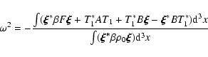
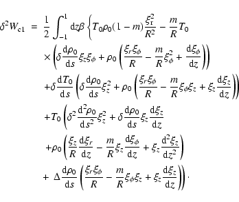
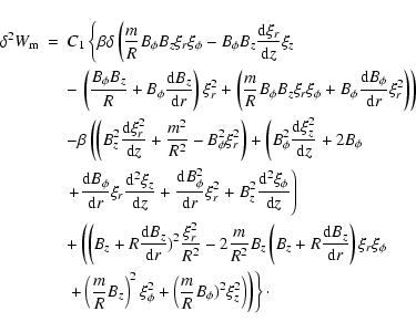
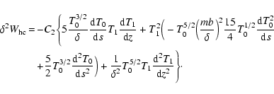
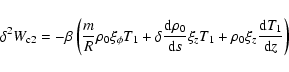
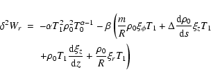
From the procedure described above and extensively exemplified in Paper I, we can obtain - lengthly but in a straightforward way - the explicit terms for the energy principle given in Eq. (10)

$$\delta^{2} W_{\rm p}= \delta^{2} W_{\rm c}+\delta^{2} W_{\rm m}+\delta^{2} W_{\rm hc}+\delta^{2} W_{\rm r}$$

where the right side of the equation corresponds to the compressional, magnetic, heat conduction, and radiative contributions,respectively. The compressional term $\delta^{2} W_{\rm c}=\delta^{2} W_{\rm c1}+\delta^{2} W_{\rm c2}$ has an additional contribution ( $\delta^{2} W_{\rm c2}$) with respect to Bernstein's principle:

$$\delta^{2} W_{\rm B}= \delta^{2} W_{\rm c1}+ \delta^{2} W_{\rm m}$$

$$\begin{eqnarray*}\delta^{2} W_{\rm c1} &=&\frac{1}{2}\int_{-1}^{1}{\rm d}z \beta... ...frac{{\rm {\rm d}}\xi_{z}}{{\rm d}z}\right) \right)\cdot \right. \end{eqnarray*}$$

The magnetic contribution is:

$$\begin{eqnarray*}\delta^{2} W_{\rm m}&=&C_{1}\left \{ \beta \delta \left(\frac{m... ...rac{m}{R}B_{\phi})^{2} \xi_{z}^{2}\right) \right) \right\}\cdot \end{eqnarray*}$$

The heat conduction term results:

$$\begin{eqnarray*}\delta^{2} W_{\rm hc}&\!\!=\!\!&-C_{2}\Bigg\{5\frac{T_{0}^{3/2}... ..._{0}^{5/2}T_{1}\frac{{\rm d}^{2}T_{1}}{{\rm d}z^{2}}\Bigg\}\cdot \end{eqnarray*}$$

The new compressional contribution is expressed as:

$$\delta^{2} W_{\rm c2}=-\beta \left(\frac{m}{R} \rho_{0}\xi_{\... ...i_{z}T_{1}+\rho_{0}\xi_{z}\frac{{\rm d}T_{1}}{{\rm d}z}\right)$$

and the term associated with radiation was:

$$\begin{eqnarray*}\delta^{2} W_{r}&=&-\alpha T_{1}^{2}\rho_{0}^{2}T_{0}^{\alpha-1... ...\rm d}\xi_{z}}{{\rm d}z}+ \frac{\rho_{0}}{R} \xi_{r}T_{1}\right) \end{eqnarray*}$$

where the following changes were made:

$$\begin{eqnarray*}\rho&\rightarrow\frac{\rho}{\rho_{t}};\quad T\rightarrow\frac{T... ...\chi T_{\rm t}^{\alpha+1}\rho_{\rm t}^{2}L/m_{\rm p}^{2}\right), \end{eqnarray*}$$

$S=\Delta L$ and the non-dimensional constants:

$$C_{1}= \rho_{\rm t}^{2}T_{\rm t}^{\alpha+1}B_{0}^{2}/(\mu_{0}... ... C_{2}=c T_{\rm t}^{\frac{7}{2}-\alpha}/(S^{2} n_{\rm e}^{2}).$$

were used. All the quantities were defined as in Paper I.

References

• Arfken, G., & Weber, H. 1995, Mathematical methods for physicists (San Diego: Academic Press) (In the text)
• Aschwanden, M. J. 2004, Physics of the Solar Corona (New York: Springer-Verlag) (In the text)
• Belien, A. J. C., Poedt, S., & Goedbloed, J. P. 1997, A&A, 322, 995 [NASA ADS] (In the text)
• Bernstein, I. B. 1958, PhRv, 109, 10 [NASA ADS] (In the text)
• Costa, A., & González, R. 2006, A&A, 458, 953 [NASA ADS] [CrossRef] [EDP Sciences] (In the text)
• Costa, A., González, R., & Sicardi Schifino, A. C. 2004, A&A, 427, 353 [NASA ADS] [CrossRef] [EDP Sciences] (In the text)
• Freidberg, J. P. 1982, Rev. Mod. Phys., 54, 3 [CrossRef] (In the text)
• Galindo Trejo, J. 1987, SoPh, 108, 265 [NASA ADS] (In the text)
• Goedbloed, J. P., & Halberstadt, G. 1993, A&A, 280, 647 [NASA ADS] (In the text)
• Goossens, M., Andries, J., & Aschwanden, M. J. 2002, A&A, 394, L39 [NASA ADS] [CrossRef] [EDP Sciences] (In the text)
• Halberstadt, G., & Goedbloed, J. P. 1994, A&A, 286, 275 [NASA ADS] (In the text)
• Heyvaerts, J., & Priest, E. R. 1983, A&A, 117, 220 [NASA ADS] (In the text)
• Linton, M. G., Longcope, D. W., & Fisher, G. H. 1996, ApJ, 469, 954 [NASA ADS] [CrossRef] (In the text)
• Nakariakov, V. M., Roberts, B., & Murawski, K. 1997, SoPh, 175, 93 [NASA ADS] (In the text)
• Priest, E. R. 1982, Solar Magneto-hydrodynamics (Boston: Publishing Company) (In the text)
• Raadu, M. A., Schmieder, B., Mein, N., & Geesztelyi, L. 1988, A&A, 197, 289 [NASA ADS] (In the text)
• Raadu, M. A. 1972, SoPh, 22, 425 [NASA ADS] (In the text)
• Roberts, B. 2000, SoPh, 193, 139 [NASA ADS] [CrossRef] (In the text)
• Ruderman, M. S. 2007, SoPh, 246, 119 [NASA ADS] (In the text)
• Sicardi Schifino, A. C., Costa, A., & Ferro Fontán, C. 1991, JMP, 32, 1350 [NASA ADS] [CrossRef] (In the text)
• Sturrock, P. A. 1994, Plasma Physics, An Introduction to the Theory of Astrophysical, Geophysical and Laboratory Plasmas (Cambridge University Press) (In the text)
• Van Doorsselaere, T., Andries, J., Poedts, S., & Goossens, M., 2004, ApJ, 606, 1223 [NASA ADS] [CrossRef] (In the text)
• Vrsnak, B., Ruzdjak, V., & Rompolt, B. 1991, SoPh, 136, 151 [NASA ADS] (In the text)